Periodic Structures and Symmetries in the Natural Numbers Modulo 12

The number 12 is a superior highly composite number divisible by 2, 3, 4, and 6. Analyzing natural numbers through their prime factorization reveals striking patterns and symmetries. The duodecimal system, based on 12, provides a natural framework for structuring natural numbers into periods and groups with similar properties. These structures offer an intuitive perspective on the behavior of the divisor and sigma functions and on residue-class constraints relevant to Goldbach-type decompositions. Furthermore, they help to interpret observed patterns in prime gaps, accounting for the prominence of certain gaps and suggesting empirical trends. This article does not claim new theorems in analytic number theory. Its contribution is a unified mod‑12 framework that brings together several classical facts and makes certain structural regularities visually and arithmetically explicit.

The number 12 is a superior highly composite number [1, 2, 7] divisible by the numbers 2, 3, 4, and 6. Superior highly composite numbers are natural numbers which have comparably many divisors. Small examples are 6 and 12, and many further examples such as 60, 120, 360, and 5040 are multiples of 12. The 12 and its divisors are ideal for dividing 60 seconds or minutes, 24 or 12 hours and 360° into smaller natural numbers / segments.

Superior highly composite numbers (= n in the formula below) are those positive integers for which there is a positive exponent ε such that:

d(n) = number of divisors for the natural number n

k = natural number > 1

Example: 12 has 6 divisors (1, 2, 3, 4, 6, 12). 6 / √12 = 1.732… which is larger than 4 / √6 = 1.633… or 12 / √60 = 1.549…

Thanks to documented evidence of the Egyptians' use of sundials, most historians credit them with being the first civilization to divide the day into smaller parts. As early as 1500 B.C., the Egyptians had developed a more advanced sundial. A T-shaped bar placed in the ground; this instrument was calibrated to divide the interval between sunrise and sunset into 12 parts. This division reflected Egypt's use of the duodecimal system (base 12). The Babylonians made astronomical calculations in the sexagesimal system (base 60) they inherited from the Sumerians, who developed it around 2000 B.C. Although it is unknown why 60 was chosen, it is notably convenient for expressing fractions, since 60 is the smallest number divisible by the first six counting numbers as well as by 10, 12, 15, 20, and 30 [3].

But in the modern world, the decimal system later prevailed, which was developed in the Indian numeral script as positional numeral system, passed on to European countries through Arabic mediation, and is now established worldwide as an international standard. Anthropologically, the emergence of the decimal system is associated with the 5 fingers of the two human hands. These served as counting and calculating aids [4].

In addition to other persons, Professor of mathematics, Alexander Aitken (1 April 1895 – 3 November 1967), was a strong advocate for changing our entire counting system from decimal to be duodecimal (base 12) [5]. He was one of New Zealand's most eminent mathematicians.

Even Leibniz noted that an advantage of duodecimal is that it allows for divisions by 2, 3, 4, and 6. He also described algorithms for converting decimal numbers into duodecimal [6].

These are the well-known advantages of the duodecimal system based on 12. In addition, the number 12 and the duodecimal system have other fundamental properties, which are presented and explained in this article.

Natural numbers form the basis of mathematics and natural sciences. Every natural number is either a prime number or can be decomposed into a product of prime numbers. Natural numbers are therefore characterized by the type and number of their divisors and prime factors.

The divisor sum Sigma(n) of a natural number n is the sum of all divisors of this number, including one and the number itself. The number 6 has the divisors 1, 2, 3 and 6, where Sigma(6) = 1 + 2 + 3 + 6 = 12

The Sigma(n) function is known as the divisor sum function and is an important number-theoretic function.

A striking pattern becomes visible when the natural numbers are organized according to their residue classes modulo 12. This pattern becomes apparent when looking at the divisor sums of all natural numbers.

The starting point for this investigation was the Lagarias inequality, through its well-known equivalence to the Riemann hypothesis [7].

Jeffrey Lagarias proved that the Riemann hypothesis is equivalent to the statement that:

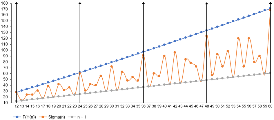
To explore this further, the values of Sigma(n) and the comparison function F(H(n)) on the right-hand side were plotted for the first natural numbers. The Sigma function fluctuates considerably, but the multiples of 12 usually attain the highest values in the plotted range (Figure 1 near here).

Figure 1

Sigma(n) versus n in intervals of 12

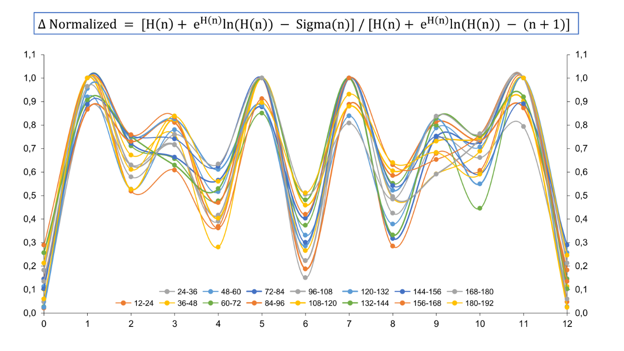
Since this function grows rapidly, the values of Sigma were normalized and superimposed in intervals of 12, yielding the following figure, which already exhibits a degree of symmetry. Since the intervals are delimited by multiples of 12, Group 12 is repeated as Group Zero. Numbers from 12 - 192 were used for the following figures (Figure 2 near here). No implication for the truth of the Riemann Hypothesis is claimed. The Lagarias inequality is used solely as a normalization benchmark.

Figure 2

Normalized Sigma values versus Group number in intervals of 12

The structure becomes more apparent when one considers the mean values, even over the relatively small range n = 12 - 192 (Figure 3 near here).

Figure 3

Averages of the normalized Sigma values versus Group number in intervals of 12.

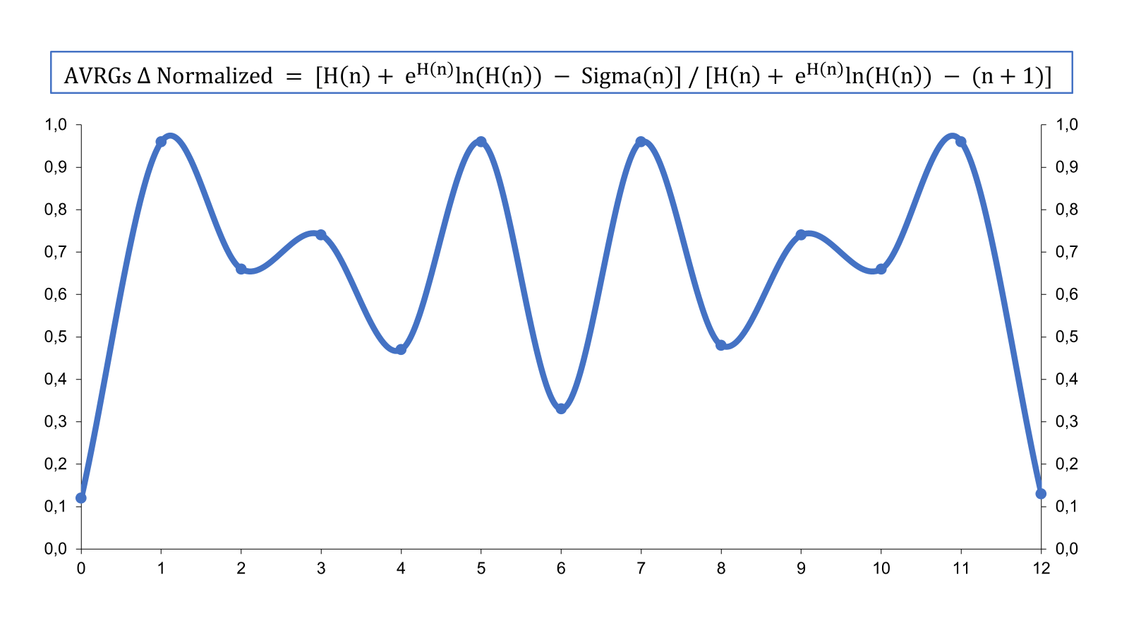
The use of mean values makes the order and symmetry of this representation particularly clear. This suggests organizing the natural numbers into Groups 1–12.

To understand the source of this structure and symmetry, it is natural to examine the numbers and their prime factorizations in Groups 1–12.

If the natural numbers are arranged not in the usual linear order on the number line, but in a table based on the duodecimal system, the following representation is obtained for the numbers from 1 to 192 (Table 1 near here).

Apart from the primes 2 and 3, every prime (RED) must lie in one of the columns 1, 5, 7, or 11 modulo 12. In this type of listing, the admissible locations of twin-prime configurations become immediately apparent.

If the natural numbers from n = 1 to 192 are arranged one below the other in intervals of 12 as above, but instead of the numbers the corresponding prime factorization is listed, a clear structural distinction between the columns (Groups 1–12) becomes apparent. The first row lists the Group labels rather than prime factorizations. The subsequent rows, beginning with the interval 13–24, are referred to as the Periods of the table (Table 2 near here).

Below are structural properties of the residue classes modulo 12, formulated in terms of prime factorization.

Structural properties of the residue classes modulo 12:

• Groups 1, 5, 7, 11: consist of prime numbers or products of prime factors starting with 5
• Groups 2 and 10: consist of integers divisible by 2 but not by 3 or 4
• Groups 3 and 9: consist of odd integers divisible by 3
• Groups 4 and 8: consist of integers divisible by 4 but not by 3
• Group 6: consists of integers divisible by 2 and 3 but not by 4
• Group 12: consists of integers divisible by 12, hence with at least two factors of 2 and at least one factor of 3, while the exponents of these factors may be arbitrarily large

Proofs via Congruence Modulo 12 (Groups 1–12):

All statements above follow from the factorization 12 = 2² · 3. Working modulo 12 encodes, at once, an integer’s parity, its divisibility by 3, and whether it is divisible by 4. Thus, the Group of a number - its residue class mod 12 - already tells us which small prime factors are forced or forbidden:

• Groups 2 and 10 (≡ 2, 10 mod 12): numbers are even but not divisible by 4 and not by 3.Therefore they have exactly one factor 2 and no factor 3
• Groups 4 and 8 (≡ 4, 8 mod 12): numbers are divisible by 4 and not by 3.Therefore they have at least two factors 2 and no factor 3
• Groups 3 and 9 (≡ 3, 9 mod 12): numbers are divisible by 3 and odd.Therefore they have at least one factor 3 and no factor 2
• Group 6 (≡ 6 mod 12): numbers are divisible by 6 but not by 4. Therefore they have exactly one factor 2 and at least one factor 3
• Group 12 (≡ 0 mod 12): numbers are divisible by 12. Therefore they have at least two factors 2 and at least one factor 3, with no upper bound on the exponents
• Prime Groups 1, 5, 7, 11 (≡ 1, 5, 7, 11 mod 12): numbers are odd and not divisible by 3.Therefore these are the only classes that can contain primes ≥ 5; moreover, any product formed solely from primes ≥ 5 also lies in (1, 5, 7, 11) mod 12

Why is the modulus 12 (i.e., arranging numbers in 12‑intervals) particularly effective at revealing this structured prime‑factor pattern?

If the natural numbers are arranged in intervals of 6 (base 6), then the above Groups 6 and 12, 4 and 10, or 2 and 8 fall into the same Group, although they have distinctly different properties, as shown above. Comparable distinctions between residue classes are less transparent when the numbers are arranged in intervals of 8, 10, or 30; this comparison is illustrated later in this article.

Only numbers in Group 12 (i.e., the multiples of 12) can contain the smallest prime factors, 2 and 3, in an unlimited amount. This helps explain why many familiar highly composite or superior highly composite examples, such as 60, 120, and 360, occur in Group 12.

To identify further integers with comparatively many divisors, consider the following heuristic construction: The numbers between 1 and 100 contain 50 numbers that can be divided by 2 and 33 numbers that can be divided by 3 ... Normalized to the divisor 3, these are the numbers 50 / 33 = 1.52 for the 2 and of course 33 / 33 = 1 for the 3. If we use the rounded quotients for the development of the prime factors, we get $2^2\bullet 3=12$.

Applying the above method to the prime factors 2, 3, and 5, one gets 50 / 20 = 2.5, 33 / 20 = 1.65 and 20 / 20 = 1 with the prime factor distribution of $2^3\bullet 3^2\bullet 5= 360$. Taking the prime factors 2, 3, 5, and 7, one gets 50 / 14 = 3.57…, 33 / 14 = 2.35…, 20 / 14 = 1.42… and 14 / 14 = 1 with the resulting prime factor distribution of , which is also a superior highly composite number.

And here we can also use the Lagarias inequality mentioned earlier:

If you determine the divisor sum Sigma(n) of the above numbers and set it in relation to the term on the right-hand side of the above inequality, you can estimate how "superior" these numbers are. For 5040 you get a quotient Q of 97.5%.

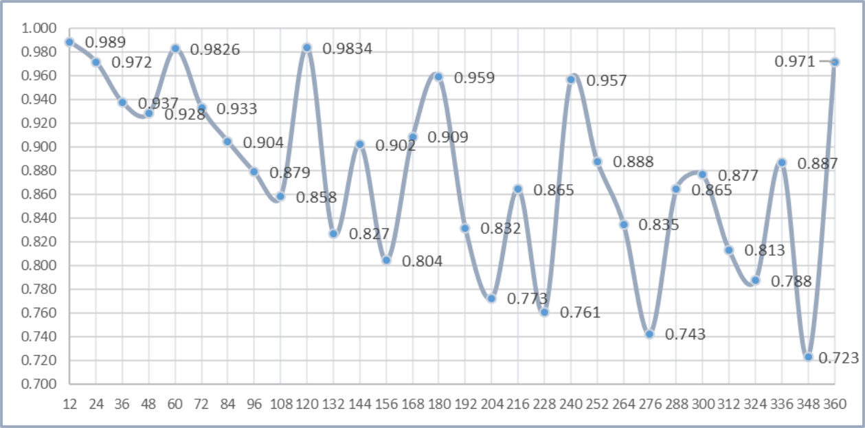
If we continue this method, we arrive at the following numbers and prime factorizations: $2^6\bullet 3^4\bullet 5^2\bullet 7^2\bullet 11=69854400$and $2^7\bullet 3^5\bullet 5^3\bullet 7^2\bullet 11\bullet 13=27243216000$. For 69854400 we get a Q value of 90.0% and for 27243216000 you get Q = 89.2%. The higher the number of smaller but also different prime factors, the higher the Q value. The Q values decrease as the number increases (here for multiples of 12), although values of 90% are still very high or good. For comparison, a plot of the Q values for the multiples of 12 from 12 to 360 is helpful. You can quickly see that the number 12 followed by 120 and 60 are closest to the function on the right-hand side of Lagaria's inequality, but also that the value for 5040 is even higher than that for 360. The lower values come from numbers that are simple multiples of 12 with one larger prime number. The figures for Group 12 show the highest Q values compared to all other Groups (Figure 4 near here).

Figure 4

Q values for the multiples of 12.

In summary, the repeating mod‑12 pattern is largely determined by the smallest prime factors, 2 and 3. These patterns start at 1 (the numbers in Group 1) and end at 12 (the multiples of 12). Thus, the structure of the natural numbers based on the number 12 / the duodecimal system is given.

In the colored tables below, you can see very clearly that the duodecimal system is particularly well adapted for simultaneously revealing divisibility by 2, 3 and 4 and therefore orders the natural numbers according to their properties (in this case their prime factor distribution).

The number system based on 24 only doubles the already existing Groups (the columns of the tables below) based on the duodecimal system and therefore offers no advantage over base 12.

All other number systems considered here (in particular bases 8, 10, and 30) reveal these divisibility patterns less uniformly and are therefore less effective for the present structural purpose (Table 3 near here).

Although the underlying congruence arguments are elementary, the resulting mod‑12 organization provides a useful framework for interpreting several familiar phenomena in elementary number theory.

For example, in the prime factorization of adjacent large numbers, no connection can be recognized at first glance:

According to the structure and the Groups of natural numbers in intervals of 12, a connection can be seen here very quickly after all:

• $2^{50}\bullet 3^{30}$: Obviously, this number is a multiple of ${12=2}^2\bullet 3$ and therefore belongs to the Group 12
• The next number above must therefore belong to Group 1 (the Group following Group 12) and could be a prime number. If not, it should only have relatively few divisors / prime factors (≥ 5)
• Then logically follows a number of Group 2, with at most one prime factor 2 and no prime factor 3
• And the fourth number belongs to Group 3, with at least one prime factor 3 (and of course no prime factor 2, as it is odd)

The same is the case for neighboring numbers in other Groups:

• The first number contains the prime factor 2 twice but no prime factor 3, so it should belong to Group 4 or 8.
• The next number contains the prime factor 3 twice (and of course no prime factor 2). It can therefore only be a number from Group 9 (and not Group 3), as Group 9 follows Group 8. Group 4 is followed by Group 5.

It is well known that several statistical models successfully describe aspects of the distribution of primes, even though the primes themselves are determined arithmetically rather than generated stochastically [8]. The next example shows that this seems to be the case for all natural numbers in their respective Groups. The distribution of properties, in this case the number and type of prime factors and divisors of the numbers in the same Group, is subject to strong fluctuations. However, if you look at the mean values of these properties in larger sets of numbers, these values are again very uniform, as can be seen from the symmetries of the similar Groups (with the axis of symmetry at Group 6, see the following diagram below). This structure and the associated symmetries can be easily recognized in the graphical representation of the divisor and sigma functions. The pattern in the numbers is repeated in intervals of 12.

This is particularly evident when intervals of 12 are superimposed for the above-mentioned function and the average values are calculated. Even intervals of 12 from 12-996 are sufficient for this.

The result for the divisor function is shown in the diagram below. It shows the average number of non-trivial divisors of all numbers when they are superimposed in intervals of 12. The results for the numbers 12-24, 24-36, 36-48, … up to 984-996 are shown as average values for the Groups 0-12. Group Zero here is a repetition of Group 12 as the interval limits are always multiples of 12 (Figure 5 near here).

Figure 5

Averages Divisor function values versus Group number for intervals of 12 from 12-996.

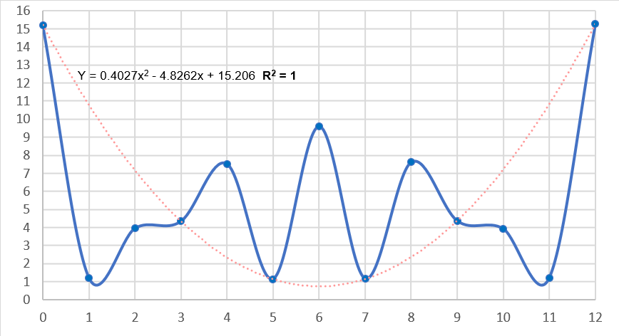
As expected, the numbers in Groups 6 (the odd multiples of 6) and 12 (the even multiples of 6) show the highest average number of divisors and the structure and symmetry of the Groups is clearly visible. A closer inspection of the plotted averages suggests an additional quadratic trend together with approximately linear segments of slopes near +/- 2 and +/- √2; these features are empirical and are not asserted here as exact laws. The values and symmetries in the diagram above suggest that prime numbers in the Groups 1, 5, 7 and 11 occur with approximately the same probability in each Group. For smaller ranges, however, Group 1 may appear to have fewer primes than the others due to the presence of prime squares, which reduce the count of distinct primes. This effect diminishes for larger ranges as prime squares become increasingly rare. These clear periodic structures and symmetries in the graphical representation of the divisor and sigma function, based on the duodecimal system, provide a compact synthesis of several classical results and make their interrelations visually transparent.

This viewpoint also clarifies in which mod‑12 residue classes special forms such as $2^n-1$ and $2^n+1$ can occur. Mersenne primes of the form $2^n-1$ belong to Group 7, as the term $2^n$(for n > 1) without the prime factor 3 only occurs in Groups 8 or 4. However, this should also apply to prime numbers of the form $2^n+1$ as these numbers should occur with the same probability in Group 5. Although the set of prime numbers from n = 3-100000 is still comparatively small, it contains 5 Mersenne primes in Group 7 as well as 5 prime numbers of the form $2^n+1$ in Group 5. This is due to the equal distribution of the terms $2^n$(for n > 1) in Groups 4 and 8. Even for the very small set of numbers from n = 1-192 in Table 2 on page 5, you can see that these terms seem to alternate in these Groups. The terms $2^2, 2^4, 2^6$ in Group 4 and $2^3, 2^5, 2^7$ in Group 8. A similar pattern can also be observed for the terms $3^n$in Groups 3 and 9

In this framework, the classical observation that every prime $p>3$ satisfies $p\equiv \pm 1 mod\mathrm{ }6$ appears naturally. This term is well known, but its underlying cause lies in the structure of the duodecimal system. While the congruence $p^2\equiv 1 mod 12$ is also well known, the observation that all such squares belong to Group 1 highlights the particular usefulness of modulus 12 for organizing these divisibility patterns.

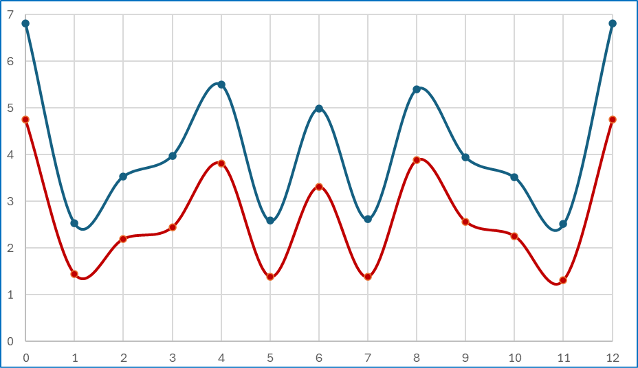
A similar structure also results if you superimpose the number of prime factors (Ω function) of all numbers in intervals of 12 and determine the average values. To see how these patterns / curves change for larger numbers and sets of numbers, the very small number interval of n = 1-192 (red curve) was chosen on the one hand and, for comparison, an interval of significantly larger numbers from n = 123456781 to 123457788 (blue curve with 1007 numbers). As shown in the diagram below, the symmetries of the Groups can be recognized in the same way and you can see an overall increase in the values with increasing numbers, without the shape of the curve changing significantly. Average number of prime factors per number versus Group number (Figure 6 near here).

Figure 6

AVRGs Omega(Ω) function values for different number intervals versus Group number

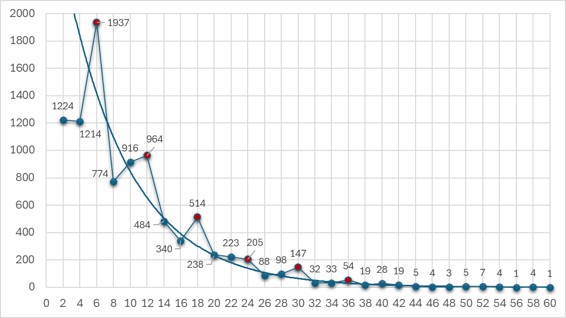
In addition, the restriction that prime numbers can only occur in Groups 1, 5, 7, and 11 introduces a clear structure in their distribution over larger intervals (e.g. from n = 3-100000). The most frequent gap between consecutive primes is 6, followed by gaps of 2 and 4. For example, in the interval n = 3-100000, among 9590 primes, 1937 exhibit a gap of 6 to the next prime. Gaps of 2 and 4 occur at roughly half this frequency, as expected from the modular arrangement of Groups 1, 5, 7, and 11. Compared to gaps of 2 and 4, gaps of 6 are about twice as frequent because they arise from transitions between Groups 1 and 7, 5 and 11, 7 and 1 (e.g., 13), and 11 and 5 (e.g., 17). Gaps of 2 or 4 are only possible between primes in Groups 5 and 7, 11 and 1 (e.g., 13), or 1 and 5, 7 and 11, making them inherently less likely (Figure 7 near here).

Moreover, since these Group transitions occur at every multiple of 6, larger gaps such as 12, 18, 24, and 30 originate from the same structural principles as gap 6. Consequently, the observed prominence of gaps that are multiples of 6 appears consistent with the underlying residue-class structure; however, no asymptotic equivalence claim is proved here. These structural relationships also explain the peak values (shown in red) for multiples of 6 in the accompanying graph. In addition, differences in the probability densities of gaps such as 8 versus 10 can generally arise from the varying distribution of prime and composite numbers within those gap distances, which influences the likelihood of consecutive primes occurring at those distances. Based on the Group structure found, varying occurrences of composites at those distances prevent the formation of certain prime gaps and seem to be the main reason for the observed differences.

Figure 7

Number of prime gaps versus gap length for the numbers 3-100000.

These relationships are empirically illustrated by computations on number intervals up to 100 million [9]. The table below presents the probability densities for prime gaps from 2 to 12 across several intervals (Table 4 near here).

It is clearly visible that the prime gap 10 is more frequent than expected compared to the prime gap 8, which is somewhat counterintuitive. Prime gaps 2 and 4 have, apart from small fluctuations, the same value due to structural reasons in the duodecimal system. The data also suggest that the ratio of the probability densities for prime gaps 12 and 6 increases consistently toward the limiting value 1. In contrast to prime gaps, the distribution of gaps between consecutive Prime Group Composite numbers (PGCs) like 25 or 35 behaves quite differently, as expected. Here, gaps of 2 and 4 dominate overwhelmingly. In the largest interval analyzed, these two gaps together account for nearly 80% of all gaps, while large gaps become exceedingly rare. For example, gap 20 occurs only 17 times in the 1-10 million range. This trend is consistent with the structural hypothesis: as the range expands, short gaps (2 and 4) become increasingly dominant, while longer gaps become rarer [9] (Table 5 near here).

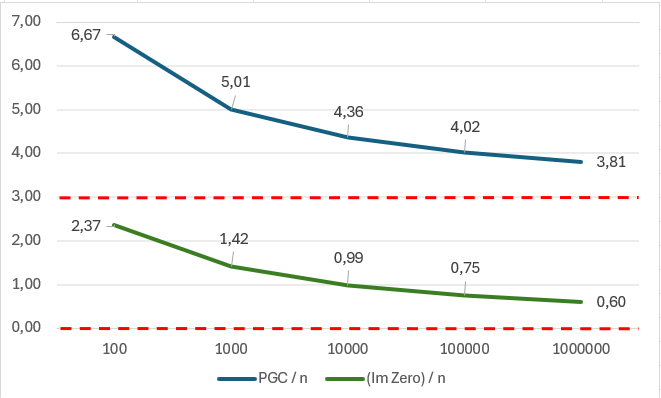
Prime Group Composite numbers (PGCs) form a complementary set to primes and together make up one-third of all natural numbers. The decrease in their average gap with increasing range invites comparison with other decreasing-spacing phenomena, such as the normalized spacing of non-trivial zeros of the Riemann Zeta function; the comparison here is heuristic rather than structural. Both PGC values and the imaginary parts of the Riemann Zeta zeros exhibit similar convergence behavior when normalized by their index, with PGC / n approaching 3 and the imaginary parts / n tending toward zero (Figure 8 near here). Both display a qualitative decay reminiscent of the function $1/\mathrm{ }\mathrm{l}\mathrm{n}\left(\mathrm{l}\mathrm{n}\right(n\left)\right)$.

Figure 8

Average gap length between PGCs and the imaginary parts of Riemann Zeta zeros

In summary, this analysis provides a coherent structural interpretation of the empirically observed distribution of prime gaps and connects these patterns to the mod‑12 organization of the natural numbers.

An especially striking empirical observation emerges when considering the sequence of all natural numbers that belong to the four prime Groups 1, 5, 7, and 11 - including composite numbers such as 25 or 35. If we build a series in blocks of four consecutive prime Group numbers, the following structure results, once again demonstrating the importance of using intervals of 12.

Calculating this sum up to the last complete 12‑interval ending at 300000 (i.e., through 25000 blocks, with the final Group 11 term 299999) gives

which agrees with π to within about 1.00000000 · 10^-5. This rapid numerical convergence is striking. At present, however, the identification of π as the limiting value should be regarded as an empirical observation rather than a proved result.

Finally, the significance of the number 12 and the multiples of 12 can also be seen in the Riemann Zeta function: The values for odd negative integers always seem to be rational numbers with a multiple of 12 in the denominator, sometimes even with the number 12 itself, e.g. for -1 or -13 the value is -1/12. If you take a closer look at these denominators for the range from -1 to -99, you can see that the number 12 seems to play a role in many respects. This is recorded here as an empirical pattern relevant to the mod‑12 perspective, not as a new theorem. Here is the graph with the natural logarithms of the denominators (Figure 9 near here).

Figure 9

Natural logarithms of the denominator of Riemann Zeta values for odd negative integers.

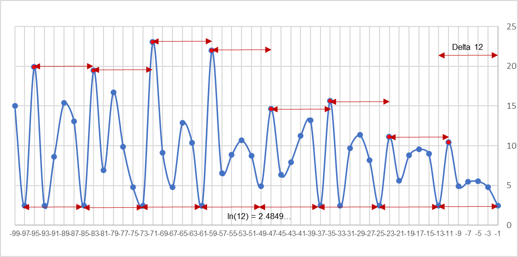
Exploring the natural numbers through a mod‑12 (duodecimal) grouping turns out to be remarkably informative. This representation makes several divisibility constraints (especially by 2, 3, and 4) visible at a glance and reveals clear “group signatures” in plots of divisor-related functions. While many individual ingredients are classical, the mod‑12 period-folding viewpoint provides a compact synthesis and leads to a rapidly convergent series built from the residue classes 1, 5, 7, 11 (mod 12) whose partial sums appear numerically to approach π.

The Goldbach conjecture is one of the unsolved problems in number theory. It states that every even natural number greater than 2 is the sum of two prime numbers.

If you apply the structure found in the natural numbers to the so-called Goldbach decomposition, you obtain a structured distribution in the number of prime number pairs per every even number depending on the Group number. This distribution is also known as the Goldbach comet and shows particularly high values for multiples of 6

This structure results if the above values are assigned to the even Groups in the Periodic System of the natural numbers (2, 4, 6, 8, 10, and 12). Particularly high values result for numbers in Groups 6 and 12 (Figure 10 near here).

Figure 10

The Goldbach comet for intervals of 12 from 98-300 versus Group number.

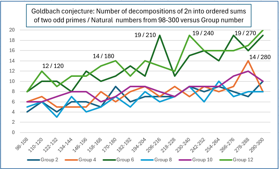
It is also already known that the above distribution for larger intervals seems to give slightly higher values for the multiples of 6 + the number 4 than those of 6 + the number 2. This can also be seen in the mean values of Groups 2, 4, 8 and 10 over the very small number range 98-300 in the diagram above. The numbers "multiples of 6 + 4" correspond to numbers in Groups 4 and 10 and the numbers "multiples of 6 + 2" correspond to numbers in Groups 2 and 8.

In contrast to the numbers in Groups 4 and 10, the numbers in Groups 2 and 8 directly follow the possible prime numbers in Groups 1 and 7. This eliminates the combination “prime number + 1” as a prime number pair in the numbers in Groups 2 and 8 as 1 is not a prime number. The difference between these Groups in the diagram above is therefore not very large and is usually only about 1.

The distances to the prime number Groups are the same in both directions for the numbers in Groups 6 and 12. The values for these Group numbers in the diagram above are almost the same on average. Only numbers of the Groups 6 and 12 have a divisor and prime factor of 3 in addition to the 2.

In principle, numbers in Group 12 can be formed by combining prime numbers from Groups 1 and 11 and combinations from Groups 5 and 7. For numbers in Group 6, these are combinations of prime numbers from Groups 1 and 5 as well as 7 and 11. This means that the probability of prime number pairs for these numbers is significantly higher (about twice as high) than, for example, for numbers in Group 4, for which only combinations from prime number Groups 5 and 11 are possible.

The diagram above also shows that numbers in Groups 6 and 12 reach peak values if they contain the prime factor 5 in addition to the prime factors 2 and 3. These numbers, such as 120, 180, 210, 240, and 270, all contain the prime factor 5 and often have a difference of 30 to the next peak number.

To illustrate the above relationships, here are tables of the prime number Groups for the number 120 (peak number) compared to the number 108 (no peak number) (Table 6 near here).

For the number 120, there are significantly more prime number pair constellations than for the number 108. The peak values for the numbers in Groups 6 and 12 appear to be based on many small and preferably different prime factors, for example $120=24 \bullet 5=2\bullet 2\bullet 2\bullet 3\bullet 5$. For larger peak values, the numbers that also contain the prime factor 7 in addition to the prime factors 2, 3 and 5 also appear to be relevant.

This may help explain why 210 is the first number to have 19 prime number pairs ($210=2\bullet 3\bullet 5\bullet 7).$ Also the number 280 (Group 4) in the diagram above shows a comparatively high number of prime number pairs and it also contains a high number of small and different prime factors: $280=2\bullet 2\bullet 2\bullet 5\bullet 7$.

This also applies to the numbers 360 in comparison to 348, and 5040 in comparison to 5028. In contrast to the number 5040, the number 5028 does not have the prime number factors 5 and 7 and therefore significantly fewer matching prime number combinations / pairs (Table 7 near here).

For example, the combination of the prime numbers 5003 and 37, 4993 and 47, 4973 and 67, as well as 4951 and 89 results in the sum 5040, while the sums of the numbers 5003 and 25, 4993 and 35, 4973 and 55, as well as 4951 and 77 result in the number 5028. But these numbers are not prime number pairs, and the number 5028 has comparably few and also larger prime factors $(5028=12\bullet 419)$. For even numbers that do not contain prime factors 5 and 7 in addition to 2 and 3, there are fewer possible prime number pair combinations because some prime numbers are combined with products of prime factors ≥ 5 such as 25, 35, 55 or 77 and therefore do not lead to any further prime number pairs.

Last but not least, the following table lists the numbers in successive 12‑intervals (Periods) arranged by Groups 1-12 and displays a factor-cofactor decomposition that highlights how composite numbers are generated from small factors (especially 2 and 3) within each Group. For clarity, primes are shown in red as the number itself, while composites are written in the form ‘smallest factor · cofactor’ (e.g., 8 is written as 2·4 rather than its full prime factorization 2³). One also sees immediately why numbers in Groups 2, 6, and 10 contain the prime 2 exactly once. (Table 8 near here). For the same neighbor-Group reason, every prime p > 3 (hence p in Groups 1, 5, 7, 11) has neighbors p − 1 and p + 1 that force a factor 3 (Group 6 or 12) and a factor 4 (Group 4, 8, or 12), so (p − 1)(p + 1) is divisible by 12 and thus p² ≡ 1 (mod 12).

References

- S. Ramanujan, Highly composite numbers, Proc. London Math. Soc. Series 2. 14 (1915), 347-409.[CrossRef]
- L. Alaoglu and P. Erdös, On Highly Composite and Similar Numbers, Trans. Amer. Math. Soc. 56 (1944), 448-469.[CrossRef]
- M. Lombardi, Why is a minute divided into 60 seconds, an hour into 60 minutes, yet there are only 24 hours in a day? Scientific American, (March 5, 2007).
- H. Haarmann, Weltgeschichte der Zahlen, C.H. Beck, München (2008), 1-29.
- B. Hay, On time, New Scientist 250, Issue 3334, (2021), 54.[CrossRef]
- L. Strickland, Leibniz on Number Systems, In: Sriraman, B. (eds) Handbook of the History and Philosophy of Mathematical Practice. Springer, Cham. (2023), 1-31.[CrossRef] [PubMed]
- J. C. Lagarias, An Elementary Problem Equivalent to the Riemann Hypothesis, American Mathematical Monthly 109 (2002), 534-543.[CrossRef] [PubMed]
- P. Erdös and M. Kac, The Gaussian law of errors in the theory of additive number theoretic functions, Amer. J. Math. 62 (1940), 738-742.[CrossRef]
- Microsoft Copilot (AI assistant), empirical determination of prime gap probability densities (gaps 2-12) based on user-provided data and computational analysis, November 2025.