Assessment of Shoreline Deformation Using InSAR and DSAS along the San Bartholomeo River, Niger Delta, Nigeria

This is an Open Access article, distributed under the terms of the Creative Commons Attribution 4.0 International License (http://creativecommons.org/licenses/by/4.0/), which permits unrestricted use, distribution and reproduction in any medium or format, provided the original work is properly cited.

Abstract

This study investigates the spatial and temporal dynamics of shoreline deformation along the San Bartholomeo River over 30 years (1995–2025) using an integrated geospatial approach. The research combines Interferometric Synthetic Aperture Radar (InSAR) and Digital Shoreline Analysis System (DSAS) techniques to quantify both vertical land motion and horizontal shoreline change. Results reveal a decline in land area from 32.622 km² (56.65%) in 1995 to 30.284 km² (52.59%) in 2025, alongside an increase in water body extent, indicating progressive shoreline retreat. Shoreline change rates varied significantly, with erosion reaching −8.04 m/yr and accretion up to 16.73 m/yr. Net Shoreline Movement (NSM) and Shoreline Change Envelope (SCE) analyses further highlighted zones of persistent erosion and high variability. InSAR-derived deformation patterns confirmed the presence of subsidence contributing to shoreline instability. The findings demonstrate that a combination of hydrodynamic forces, sediment imbalance, and anthropogenic activities drives shoreline deformation in the study area. This study contributes to improved shoreline monitoring by integrating vertical and horizontal deformation metrics, providing a robust framework for sustainable shoreline management in deltaic environments.

1. Introduction

Shorelines represent dynamic boundaries that continuously respond to environmental forcing and human activities. In deltaic environments such as the Niger Delta, shoreline deformation poses significant risks to ecosystems, infrastructure, and local livelihoods. Increasing pressures from climate variability, sediment disruption, and anthropogenic activities have intensified shoreline instability, making accurate monitoring essential (Odunuga, Oyebande, Omojola, & Adeaga, 2015; Ndubisi & Ezirim, 2021) [1, 2].

Traditional shoreline studies have largely focused on horizontal movement using optical imagery, often neglecting vertical land motion such as subsidence. However, recent advances in satellite geodesy, particularly Interferometric Synthetic Aperture Radar (InSAR), have enabled the detection of millimetre-scale ground deformation, offering new opportunities for integrated shoreline analysis. Previous studies (Vousdoukas et al., 2020; Cooper & Pontee, 2016) [3, 4] emphasize the importance of monitoring shoreline change using geospatial techniques. However, many studies neglect vertical deformation. Despite the growing application of geospatial technologies in coastal monitoring, no published study has comprehensively assessed shoreline deformation along the San Bartholomeo River using an integrated InSAR and Digital Shoreline Analysis System (DSAS) approach. Existing studies have established that coastal and shoreline terrain can be monitored using conventional techniques with sparse and discrete spatial information. However, the knowledge gap has heightened the quest for the availability of reliable spatial information needed to understand long-term shoreline dynamics and to support evidence-based coastal management in the area. Addressing this issue is critical because the consequences of coastal and shoreline changes will impact the socioeconomic realities of the communities and critical investments of operating companies in the location. Given this identified gap, this study integrates Interferometric Synthetic Aperture Radar (InSAR) and DSAS-derived shoreline metrics to assess shoreline deformation in the San Bartholomeo River, a riverine–mangrove system in the Niger Delta where persistent shoreline instability threatens coastal ecosystems, infrastructure, and the livelihoods of adjoining communities. Specifically, the study quantifies the rate, magnitude, and spatial extent of shoreline deformation over 30 years (1995–2025) using InSAR observations and DSAS statistical models. The findings provide baseline geospatial information to support sustainable shoreline management, climate adaptation, disaster-risk reduction, and coastal resilience planning in the Niger Delta.

2. Study Area

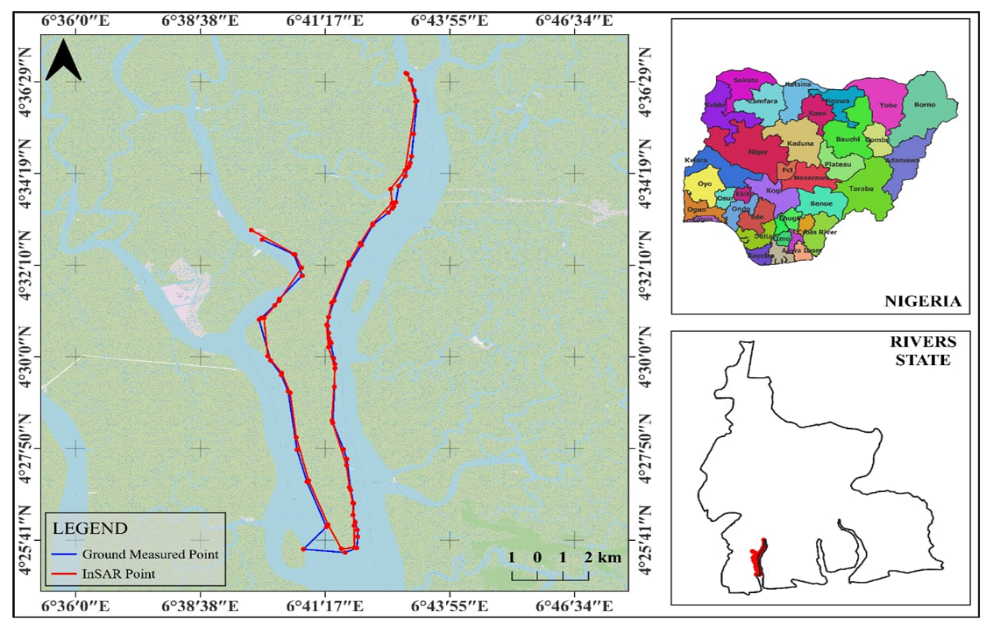
The study is located in Akuku-Toru Local Government Area of Rivers State, in the Niger Delta region of Nigeria. The area is a stretch along the San Bartholomeo River, characterized by low-lying terrain, tidal influence, mangrove vegetation, and unconsolidated sediments. These features make the shoreline highly susceptible to erosion, accretion, and subsidence. It has a shoreline that stretches approximately 41km in length and spans from a point at Ekulama I on Latitude 4° 33’ 44” N and Longitude 6° 42’ 46” E to Ekulama II on Latitude 4° 32’ 55” N and Longitude 6° 39’ 46” E. Ezekwe, Eludoyin, and Adigwu (2015) [5] explained that the area is among the swampiest of the ecological zones, under tidal influence. The vegetation around the river consists of a mangrove system intermingled with rainforest. As depicted in Figure 1, the river is economically important to Rivers State and Nigeria at large, as it hosts major flow stations, such as Ekulama I and II, which provide gas feedback to the Nigerian government-owned Bonny LNG terminal (Ezekwe et al., 2015) [5].

3. Materials and Methods

This research adopts an integrated remote sensing and Interferometric Synthetic Aperture Radar (InSAR) methodological framework to assess shoreline deformation and vertical land motion along the San Bartholomeo River. It uses a quantitative approach. Quantitative because it deals with measurable changes in shoreline position, erosion, accretion, and subsidence, and uses statistical analysis to achieve the research objectives.

3.1. InSAR Radar Data

Multi-temporal Synthetic Aperture Radar (SAR) images from satellites such as Sentinel-1, Radarsat-1, and Radarsat-2 provide raw interferometric phase data for deformation analysis. The research used satellite imagery from four distinct years (1995, 2005, 2015, and 2025) to create a comprehensive temporal dataset of shoreline changes. The selected years correspond to key periods of interest, with each dataset providing insights into both short-term and long-term shoreline dynamics. In Synthetic Aperture Radar (SAR), a satellite transmits a microwave signal toward the Earth’s surface. The signal is reflected, and the satellite records the returned wave. The Radar Signal can be represented as:

S = {A e}^{i ø}

(1)

Where:

S = Complex Radar Signal

$A$ = amplitude (depends on surface roughness, dielectric properties, etc.)

ϕ= phase of the radar signal

$e$ = exponential operator representing wave behavior

$i$ = imaginary unit, allowing 2D representation (cos + sin)

The phase is directly related to the distance between the radar and the ground target:

ϕ = \frac{4 π R}{λ}

(2)

Where:

R = range (satellite-to-ground distance)

λ = radar wavelength

3.2. Data Acquisition

3.3. Data Analysis

The raw Sentinel-1 SAR data were imported into SNAP software (Sentinel Application Platform) using the Read function, which loaded the satellite images required for further processing. InSAR processing was carried out using SNAP software to derive vertical land motion. Time-series techniques (e.g., SBAS/PSI were used to estimate deformation rates. Once the data were loaded, the next step involved generating the interferogram by comparing the phase differences between two SAR images captured at different times. This interferogram highlighted any displacement of the Earth’s surface between the two acquisition dates, providing the fundamental data for understanding shoreline deformation. Since the Sentinel-1 data is acquired in TOPSAR mode (which divides the data into multiple sub-swaths or bursts), the TOPSAR-Deburst process was applied to split the data into individual sub-swaths, allowing for more accurate and efficient analysis of the area of interest (AOI) and reducing unnecessary data.

3.4. Shoreline Extraction and Analysis

Shorelines were extracted from satellite imagery and analysed using DSAS. Key metrics include:

3.4.1. Endpoint Rate (EPR)

The EPR measures the rate of shoreline change by directly comparing the positions of the shoreline between two time periods (e.g., 1995–2005, 2005–2015, and 2015–2025). The EPR is calculated by dividing the distance between the shoreline positions at the two endpoints by the time difference.

Endpoint Rate (EPR):

\frac{D i s t a n c e}{T i m e} = \frac{E - B}{T}

(3)

Where:

E = Endpoint

B = Beginning Point

The EPR provides a simple but effective measure of the rate of shoreline movement, particularly for cases where only two points (beginning and end of the period) are available. It gives a clear snapshot of how fast the shoreline has changed over the time period in question.

3.4.2. Linear Regression Rate (LRR)

The LRR method uses a least squares regression to determine the best-fit line through the shoreline positions at each transect over time. The slope of this line represents the rate of shoreline change per year. The LRR provides a smoothed estimate of the rate of change, accounting for long-term trends in shoreline movement. It is particularly useful when there are multiple data points (e.g., multiple years) and when the shoreline has experienced fluctuating changes over time. In this study, the DSAS tool was used in ArcGIS. It is calculated for each transect between the selected years (1995–2005, 2005–2015, and 2015–2025). LRR is typically expressed in meters per year (m/yr). Mathematically, it is given as:

L = m x + b

(4)

Where:

L = The shoreline position (distance in meters, from a set baseline)

x = The date of the shoreline survey (years)

m = The calculated linear regression rate of change (slope/rate)

b = The estimated y-intercept of the regression line.

3.4.3. Net Shoreline Movement (NSM)

The NSM measures the total distance between the oldest and most recent shoreline positions along each transect. It provides a direct measure of long-term shoreline displacement, indicating whether a particular section has experienced net erosion or net accretion over the study period. Mathematically, NSM is expressed as:

N S M = S_{f i n a l} - S_{i n i t a l}

(5)

Where:

$S_{f i n a l}$ = most recent shoreline position

$S_{i n i t a l}$ = earliest shoreline position

3.4.4. Shoreline Change Envelope (SCE)

Shoreline Change Envelope measures the total range of shoreline movement, defined as the distance between the most landward and most seaward shoreline positions recorded across all time periods. It is expressed mathematically as:

S C E = S_{m a x} - S_{m i n}

(6)

Where:

$S_{m a x}$ = most seaward shoreline position

$S_{m i n}$ = most landward shoreline position

3.5. Validation

To ensure the reliability of the InSAR-derived results, a validation exercise was conducted as a crucial part of this research. It was done to verify satellite-based measurements of shoreline deformation by comparing them with on-the-ground observations. The difference between ground-measured height and InSAR-derived height was computed to assess accuracy. The height difference computation is given as;

∆ h = h_{I n S A R} - h_{G r o u n d}

(7)

Where:

$∆ h$ = difference between InSAR-derived height and ground-measured height

$h_{I n S A R}$ = InSAR-derived vertical displacement

$h_{G r o u n d}$ = Ground control measured height

3.6. Statistical Analyses

The validated ground data were integrated into the overall analysis to enhance the interpretation of the deformation patterns. Statistical analysis plays a critical role in evaluating the accuracy and reliability of geospatial datasets, particularly in deformation monitoring using InSAR and ground-based measurements. The use of Root Mean Square Error (RMSE) and other statistical indicators, such as Mean Absolute Error (MAE) and Correlation Coefficient, is essential for validating the consistency between observed and derived measurements. The Root Mean Square Error was computed to measure the square root of the average squared differences between values predicted by InSAR-derived heights and values observed from ground control points. This is given as:

R M S E = \frac{\sqrt{\sum (h_{I n S A R - h_{G r o u n d}})^{2}}}{n}

(8)

Where:

RMSE = Root Mean Square Error

$h_{I n S A R}$ = InSAR-derived vertical displacement

$h_{G r o u n d}$ = Ground control measured height

$n$ = No of points

While Mean Absolute Error (MAE) was computed to measure the average absolute difference between InSAR-derived height and observed values without squaring the errors. This is given as:

M A E = \frac{\sqrt{\sum h_{I n S A R - h_{G r o u n d}}}}{n}

(9)

MAE = Mean Absolute Error

$h_{I n S A R}$ = InSAR-derived vertical displacement

$h_{G r o u n d}$ = Ground-measured height

$n$ = No of points

On the other hand, the Correlation Coefficient was computed to measure the strength and direction of the linear relationship between ground-measured values and InSAR-derived values. It determines how strongly the two datasets are related. A high correlation coefficient indicates that InSAR results closely follow ground observations. It is given as:

r = \frac{n (\sum x y) - (\sum x) (\sum y)}{\sqrt{[n \sum x^{2} - (\sum x)^{2}] [n \sum y^{2} - (\sum y)^{2}]}}

(10)

Where:

$r$ = correlation coefficient,

$n$ = no of points

$\sum x y$ = Sum of each x-value multiplied by its corresponding y-value

$\sum x$ , $\sum y$ = the sums of each variable

$\sum x^{2}$ , $\sum y^{2}$ = the sums of squared values

This implies that when r ranges from -1(perfect negative) to +1(perfect positive), it is good.

4. Results and Discussion of Findings

The results contain tables showing the extent, rate, and magnitude of shoreline deformation

4.1. Rate and Magnitude of Shoreline Deformation

Shoreline change rates varied significantly across transects:

NSM analysis revealed cumulative shoreline retreat in several transects, while SCE indicated high variability in shoreline positions, reflecting dynamic sediment processes.

4.2. Vertical Land Motion (InSAR Results)

InSAR analysis identified zones of subsidence, which correlate with areas of high shoreline retreat. This confirms that vertical deformation contributes significantly to shoreline instability.

Maximum erosion: −8.04 m/yr

Maximum accretion: 16.73 m/yr

4.3. Statistical Accuracy Assessment

To validate the agreement between the datasets, some statistical analyses were performed: Root Mean Square Error was computed using equation 8 and the correlation coefficient in equation 10.

As discussed earlier, the Correlation Coefficient was computed to measure the strength and direction of the linear relationship between ground-measured values and InSAR-derived values. It determines how strongly the two datasets are related. A high correlation coefficient indicates that InSAR results closely follow ground observations.

The correlation coefficient ranges from -1 (perfect negative) to +1 (perfect positive), so a value close to +1 is good. The result shows that a strong positive correlation existed between ground measurements and InSAR-derived displacement values, demonstrating the high reliability of the InSAR technique.

5. Discussion on Results and Findings

The results demonstrate that a combination of natural and anthropogenic factors drives shoreline deformation. Hydrodynamic forces and sediment imbalance are primary natural drivers, while human activities such as dredging and oil exploration exacerbate deformation.

The integration of InSAR and DSAS provides a more comprehensive understanding of shoreline dynamics by capturing both vertical and horizontal changes. This approach addresses limitations in previous studies that relied solely on optical data and traditional surveying methods, which are limited to horizontal changes and are costly and time-consuming.

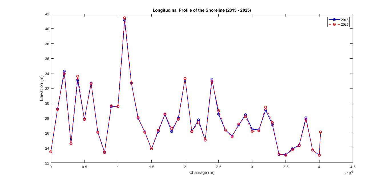
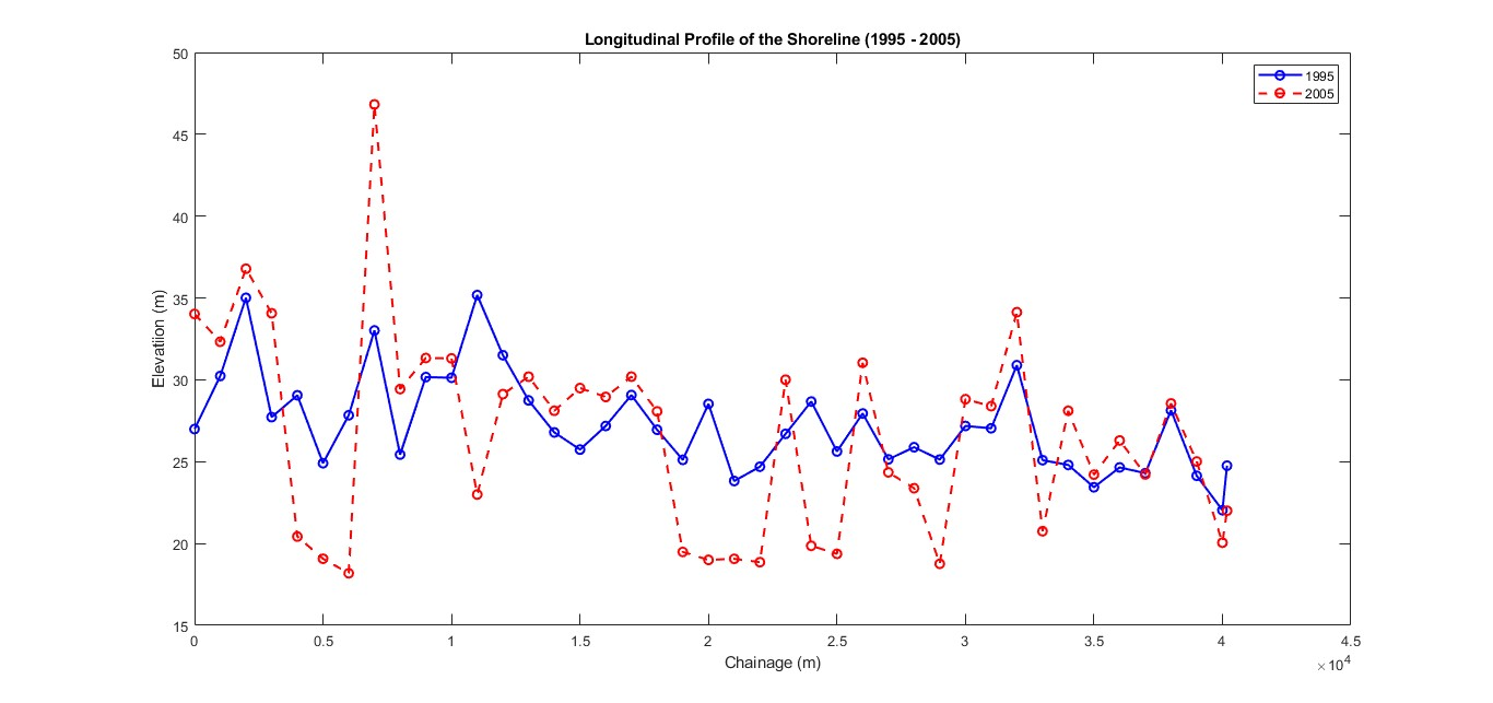
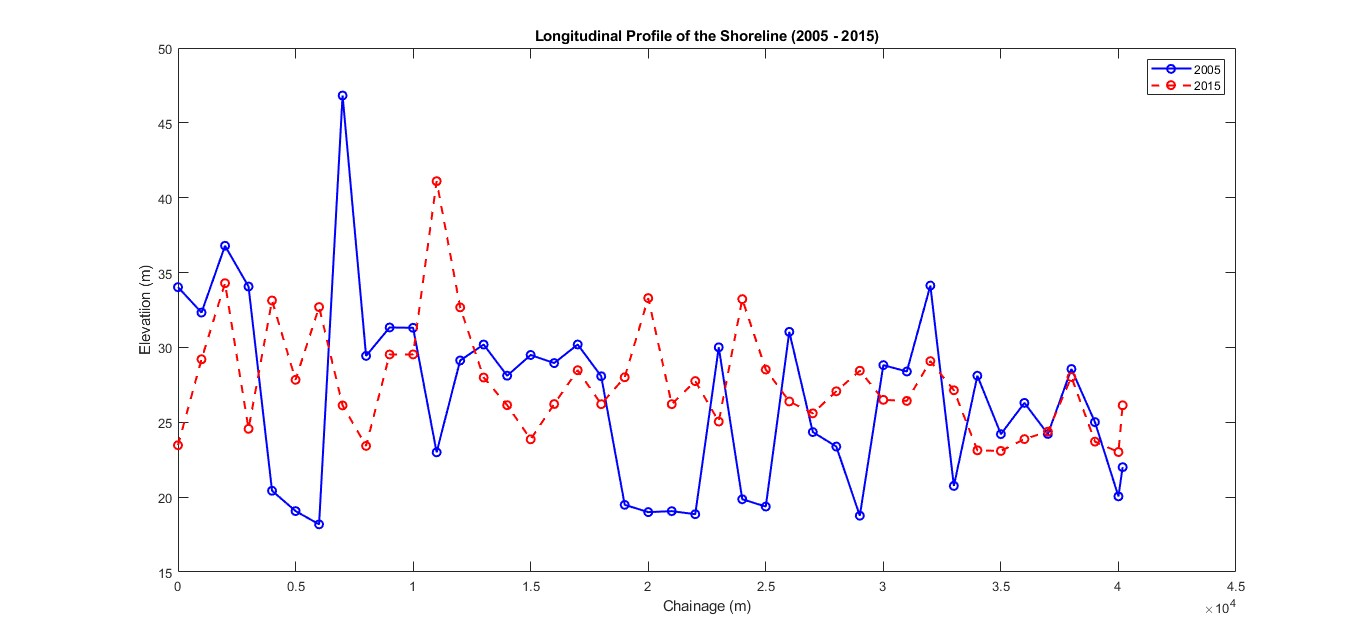
The evaluation of shoreline deformation extent, presented in Table 3, demonstrated a combination of erosion, accretion, and subsidence across the study area. Erosion was most pronounced at chainages 0+5000 and 0+6000 in 2005, where the shoreline elevation declined significantly, whereas accretion was observed at chainages 26 and 30, with elevation increases. Subsidence was also evident, particularly in zones where the shoreline consistently sank over time. These findings are consistent with other studies on shoreline dynamics in river systems, which show that shoreline deformation often results from a combination of natural processes, including sediment transport, hydrological fluctuations, and tectonic influences (Liu, Yang, Xi, Guo, & Yang, 2023) [6]. The findings of this study highlight the varying impacts of these forces along different stretches of the San Bartholomeo River, supporting previous work on the complex nature of shoreline changes in coastal and riverine areas.

The analysis of the rate and magnitude of shoreline deformation in Table 2 and Table 3 revealed that the study area experienced both high rates of erosion and significant accretion. The Linear Regression Rate (LRR) and Endpoint Rate (EPR) indicated substantial erosion in certain areas, such as Transects 1, 2, and 9, with EPR values as low as -8.04 m/yr, while other areas, like Transects 27 and 28, showed positive rates of shoreline advance, with EPRs as high as 16.73 m/yr. The classification of deformation magnitudes further revealed that high- and very-high-deformation zones were concentrated along these transects, where the most significant changes occurred. These findings align with studies by Gornitz et al. (2020) [7], who reported similarly high rates of shoreline deformation in coastal areas, where accelerated erosion is often driven by anthropogenic factors such as land-use change and river management practices. The identification of severe and extreme deformation zones in this study underscores the importance of monitoring and addressing shoreline changes in regions experiencing high rates of erosion. This study contributes to the achievement of the United Nations Sustainable Development Goals by generating geospatial evidence to support climate adaptation, sustainable coastal management, and disaster risk reduction. Specifically, the findings advance SDG 13 (Climate Action) through improved understanding of climate-induced shoreline dynamics and anthropogenic impacts. With quantitative evidence of shoreline deformation, it identifies hotspots of erosion and accretion. This will indeed support resilient land-use planning and infrastructure development in vulnerable coastal communities.

6. Conclusion

This study provides a comprehensive assessment of shoreline deformation along the San Bartholomeo River using integrated geospatial techniques. The findings highlight the importance of combining InSAR and DSAS for accurate shoreline monitoring and support evidence-based policy and Coastal Zone Management.

7. Recommendations

Continuous InSAR monitoring should be implemented along the San Bartholomeo Shoreline to detect subtle changes in shoreline position and elevation. This will provide real-time data for decision-making, particularly in areas where traditional monitoring methods are impractical due to access constraints and their cost implications.
Subsidence can exacerbate shoreline erosion and lead to infrastructural failure. It is recommended that local authorities work with oil and gas companies to monitor subsidence risks regularly and develop mitigation strategies to safeguard critical infrastructure, such as platforms and pipelines along the shoreline.
Policymakers should ensure that the potential impacts of these activities on shoreline stability are carefully assessed and mitigated through stricter regulations and monitoring.

References

Odunuga, S., Oyebande, L., Omojola, A. S., & Adeaga, O. (2015). Shoreline changes and their implications for urban infrastructure in coastal Lagos, Nigeria. Natural Hazards, 78(2), 1291–1308. https://doi.org/10.1007/s11069-015-1763-5
Ndubisi, C.C., & Ezirim, G. E. (2021). Shoreline erosion and environmental degradation in coastal communities of Rivers State. Nigerian Journal of Environmental Sciences, 15(2), 45-58.
Vousdoukas, M. I., Ranasinghe, R., Mentaschi, L., et al. (2020). Sandy coastlines under threat of erosion. Nature Climate Change, 10, 260–263. https://doi.org/10.1038/s41558-020-0697-0[CrossRef]
Cooper, J. A. G., & Pontee, N. (2016). Appraisal and evolution of the littoral ‘sediment cell’ concept in applied coastal management: Experiences from England and Wales. Ocean & Coastal Management, 135, 64–75. https://doi.org/10.1016/j.ocecoaman.2016.10.014[CrossRef]
Ezekwe, I.C., Eludoyin, O.S., & Adigwu, O. (2015). Land use dynamics and Mangrove Forest Decline in the Soku Oil and Gas Fields, Niger Delta Region of Nigeria. Journal of Geographic Thought & Environmental Studies, 2015, 13(1), 1-12.
Liu, M., Yang, Z., Xi, W., Guo, J., & Yang, H. (2023). InSAR-based method for deformation monitoring of landslide source area in Baihetan reservoir, China. Front. Earth Sci. 11:1253272. doi: 10.3389/feart.2023.1253272.[CrossRef]
Gornitz, V., Oppenheimer, M., Kopp, R., Horton, R., Orton, P., Rosenzweig, C., Solecki, W., & Patrick, L. (2020): Enhancing New York City's resilience to sea level rise and Increased Coastal Flooding. Urban Clim., 33, 100654, doi:10.1016/j.uclim.2020.100654.[CrossRef]

Article Metrics

31

Views

10

Downloads

How to Cite

                        Loading...
                    