Parametric Optimization of Thermoelastic Energy Harvesting Systems under Low-Grade Thermal Cycling

This study presents a physics-based parametric optimization framework for thermoelastic energy harvesting from cyclic temperature variations using a cylindrical AISI 4340 steel rod. The model couples thermoelastic force and displacement, Euler buckling and yielding constraints, lumped-capacitance heat transfer, and mass-power multi-objective optimization. The feasible design space was evaluated as a function of rod diameter, length, temperature change, and load-transfer parameter. The results show that Euler buckling governs the practically relevant portion of the design space at moderate temperature changes, whereas yielding becomes increasingly restrictive at higher thermal loads. The Pareto-optimal solutions exhibit a clear mass-power scaling law, with the analytical prediction P_avg ∝ m^2/3 closely reproduced by the numerical fit (n = 0.66717, R² = 0.999999). Under the baseline condition λ = 0.50, the maximum-power design produces approximately 0.16624 W, while a distance-to-ideal criterion identifies a substantially lighter compromise design with m = 223.0 kg and P_avg = 0.09231 W. Refined optimization gives λ_opt = 0.473 and P_max = 0.170454 W, indicating a power penalty of only 2.47% when the simpler λ = 0.50 condition is used. Grid-refinement tests show changes below 0.006% in maximum power and below 0.5% in the compromise-design mass between the 250 × 250 and 500 × 500 grids. The results establish compact scaling and optimization rules for balancing structural stability, thermal response, mass, and average mechanical power in thermoelastic energy-harvesting elements.

Low-grade thermal energy is widely available in industrial waste-heat streams, geothermal and solar-thermal resources, and naturally occurring temperature variations, yet a substantial fraction of this energy remains difficult to convert into useful work because of the relatively weak thermodynamic driving force associated with small temperature differences [1, 2, 3]. The recovery of such energy has therefore attracted sustained interest as a means of improving overall energy efficiency and exploiting thermal resources that are otherwise rejected to the environment.

Several technologies have been investigated for low-temperature heat conversion. Organic Rankine cycles (ORCs) can recover low- and medium-temperature heat from industrial, geothermal, biomass, and solar sources, but their practical implementation requires a working fluid, heat exchangers, pumping, expansion machinery, and careful matching between the working fluid and the heat-source temperature [2, 3, 4]. Solid-state thermal-energy-harvesting approaches provide an alternative route and include thermoelectric, pyroelectric, thermomagnetic, and thermoelastic mechanisms [1]. Experimental work has also demonstrated that appropriately designed thermal harvesters can operate under very small temperature gradients; for example, thermomagnetic energy scavenging has been demonstrated at temperature differences as low as 2 K [5]. These developments emphasize both the potential value of low-grade heat and the importance of identifying conversion mechanisms that remain effective when the available thermal driving force is limited.

Thermoelastic conversion offers a conceptually different approach because it can exploit the reversible thermal expansion and contraction of structural materials. Classical thermoelasticity establishes that a temperature change produces thermal strain, while mechanical restraint converts part or all of this strain into stress [6]. Consequently, a freely expanding member can provide displacement with negligible restraint force, whereas a fully restrained member develops thermal stress while suppressing the displacement required for mechanical work. An intermediate restraint condition can provide both force and displacement and therefore offers a potential route for extracting mechanical energy from cyclic temperature variations. Low-grade thermal-energy-harvesting literature has identified thermoelastic and thermomechanical effects among the mechanisms capable of converting temperature variations into mechanical response [1, 7]. Related studies have demonstrated thermal-to-mechanical energy conversion using thermally driven deformation, including polymer-based torsional actuators and thermally activated composite structures [8, 9]. Thermomechanical coupling has also been exploited in experimentally demonstrated energy-conversion cycles in which thermal and mechanical loading are combined to produce electrical output [10]. The use of ordinary material expansion and contraction as the basis of an alternative renewable-energy conversion concept was also investigated by Parsokhonov et al. [11].

The engineering performance of such a system cannot, however, be inferred from thermal expansion alone. Rod diameter and length simultaneously affect thermal displacement, axial force, structural mass, thermal inertia, and resistance to Euler buckling. Increasing diameter generally increases force capacity and buckling resistance but also increases the mass that must be thermally cycled. Increasing length increases the available thermal displacement but reduces buckling resistance and alters the thermal response time. Similarly, a larger temperature excursion increases the thermoelastic driving force while progressively reducing the structurally admissible region through yielding and instability. These competing effects imply that thermoelastic harvesting is intrinsically a constrained thermo-mechanical optimization problem rather than a simple maximization of thermal expansion.

A further complication is that energy per cycle alone does not determine useful performance. The time required for heating and cooling directly controls the achievable average power. Heat-transfer conditions, particularly the convective heat-transfer coefficient and the characteristic dimensions of the rod, therefore interact with structural design. This coupling makes it necessary to consider thermal dynamics, structural stability, mass, and mechanical energy within a unified framework rather than optimizing each quantity independently. The broader low-grade energy-harvesting literature similarly shows that device-level performance depends strongly on the coupling between the active conversion mechanism and heat-transfer conditions [1, 5].

Our previous work established a physics-constrained framework for modular thermoelastic energy harvesting and examined scaling and techno-economic limits associated with cyclic expansion and contraction of structural members [12]. The present study addresses a different and more focused question: how should the geometry and load-transfer condition of an individual thermoelastic rod be selected when structural stability, thermal cycling time, mass, and average mechanical power are considered simultaneously? The emphasis is therefore shifted from system-level modular energy and economic assessment toward the parametric design space, governing failure modes, and multi-objective optimization of the thermoelastic element itself.

Accordingly, this study develops a coupled analytical-numerical optimization framework in terms of rod diameter (D), length (L), temperature change (ΔT_rod), and a dimensionless load-transfer parameter (λ). The parameter (λ) represents the partition of unconstrained thermal expansion between mechanically utilized displacement and elastic restraint. Yielding and Euler buckling are imposed as structural feasibility constraints, while a lumped-capacitance thermal model is used to determine the thermal time scale and average mechanical power. The resulting formulation is used to construct the feasible (D - L - ΔT_rod) design domain, identify transitions between buckling- and yield-controlled behavior, and determine non-dominated mass-power solutions.

Three specific contributions are pursued. First, structural feasibility maps are developed to reveal how the admissible geometry changes with temperature excursion and which failure mechanism governs different regions of the design space. Second, the mass-power Pareto front is examined analytically and numerically, leading to a buckling-limited scaling relation close to (P_avg ∝ m^2/3). Third, the robustness of the optimum is evaluated with respect to convective heat transfer, numerical resolution, and the load-transfer parameter. The analysis thereby provides compact design rules for balancing structural feasibility, thermal response, mass, and average mechanical power in thermoelastic energy-harvesting elements.

2.1. Thermoelastic Rod and Load-Transfer Formulation

The energy-harvesting element is modeled as a homogeneous cylindrical rod of length L and diameter D subjected to a reservoir temperature change ΔT_R. The rod is assumed to remain within the linear-elastic regime before the imposed yielding or buckling limits are reached. For a uniform rod temperature change ΔT_rod, the unconstrained axial thermal elongation is [6]:

where α is the coefficient of thermal expansion. Free thermal expansion produces the maximum displacement but essentially no restraint force, whereas complete axial restraint suppresses useful displacement while producing the maximum elastic thermal force. To represent intermediate operating conditions, a dimensionless load-transfer parameter λ is introduced, where 0 ≤ λ ≤ 1. The mechanically available displacement is defined as:

and the corresponding axial thermal stress is:

where E is Young’s modulus. The resulting axial thermal force is:

where the cross-sectional area of the cylindrical rod is:

The physical meaning of λ, together with the principal geometric variables and the partition between mechanical displacement and elastic restraint, is illustrated in Figure 1.

Figure 1

Schematic representation of the thermoelastic rod and the load-transfer model. A cylindrical rod of diameter D and length L undergoes thermal expansion under a temperature change ΔT_rod. The load-transfer parameter λ defines the partition between mechanically utilized displacement and elastic restraint, thereby determining the axial force-displacement combination and the extractable mechanical energy.

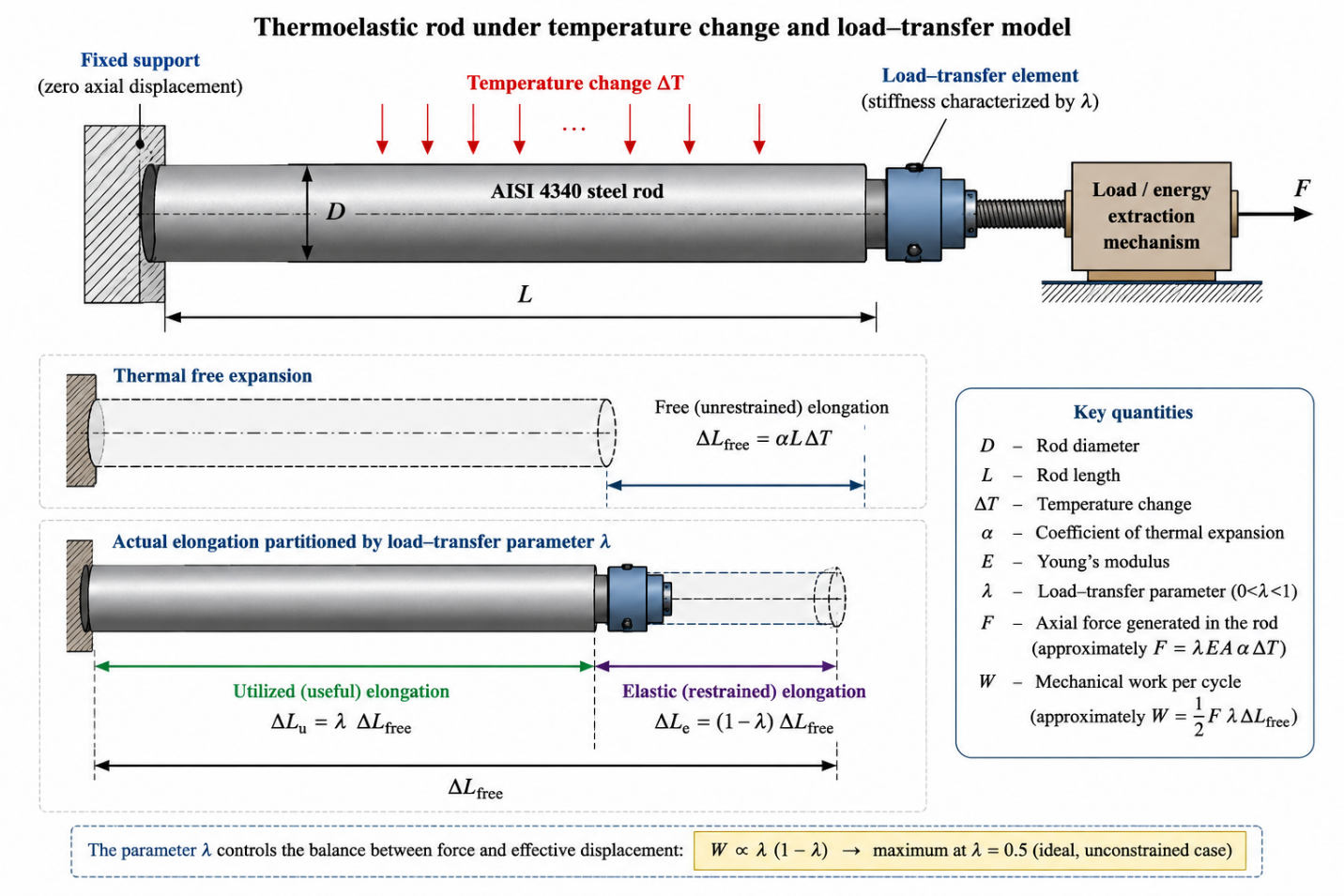
Assuming quasi-static linear loading between the unloaded and restrained states, the available mechanical work during one loading branch is approximated by the area under the force-displacement relation:

Substitution of Eqs. (1), (2), and (4) gives:

Equation (7) shows explicitly how the mechanical work depends on rod geometry, temperature change, and the load-transfer parameter. For fixed geometry and temperature, the factor λ(1 − λ) reaches its theoretical maximum at λ = 0.5. In a structurally constrained system, however, the system-level optimum need not occur exactly at λ = 0.5 because increasing λ also increases the compressive thermal force and therefore changes the admissible geometry through the buckling constraint. The material properties of AISI 4340 steel and the baseline operating and model parameters used in the calculations are summarized in Table 1.

2.2. Structural Feasibility Constraints

Two principal structural failure modes are considered: material yielding and elastic Euler buckling. Yielding is avoided when the thermal stress does not exceed the allowable stress:

where σ_y is the yield strength and SF_y is the yield safety factor. For a rod subjected to axial compression, the elastic critical buckling load is represented by the classical Euler relation [14, 15]:

where K is the effective-length factor and I is the second moment of area. For a solid circular rod:

A pinned-pinned idealization is adopted in the baseline model, corresponding to K = 1.0 [14]. The buckling feasibility condition, including the buckling safety factor SF_b, is:

These relations demonstrate the strong geometric dependence of structural feasibility. The thermal force scales with D², whereas Euler buckling resistance scales with D⁴/L². Consequently, increasing rod diameter strongly improves resistance to buckling, while increasing rod length progressively reduces the allowable compressive thermal force. This competition becomes central to the feasible-design-space analysis presented in Section 3.

2.3. Lumped Thermal-Response Model

The mechanical energy generated during a single thermal cycle does not by itself determine the useful performance of the system. Average power also depends on the time required to heat and cool the rod. The transient thermal response is therefore represented using the lumped-capacitance approximation [16, 17]. The validity of this approximation is evaluated using the Biot number:

where h is the convective heat-transfer coefficient, k is the thermal conductivity of the rod, and L_c is the characteristic length:

where V is the rod volume and A_s is the exposed heat-transfer surface area. The commonly adopted criterion Bi < 0.1 is used to ensure that internal temperature gradients remain sufficiently small for the lumped-capacitance approximation [16, 17, 18]. For the cylindrical rod:

and, assuming convection from the cylindrical surface and both end faces:

The corresponding lumped thermal time constant is:

where $\mathrm{\rho }$ is the material density and c_p is the specific heat capacity [16, 17]. Rather than assuming that the rod instantaneously reaches the reservoir temperature, a temperature-response fraction ϕ is introduced. The effective temperature change experienced by the rod is therefore:

The baseline analysis uses ϕ = 0.90, meaning that the rod is assumed to undergo 90% of the imposed reservoir temperature change during each thermal transition. For symmetric heating and cooling between the prescribed switching temperatures, the duration of each thermal leg is:

For the symmetric heating-cooling process implemented in the numerical model, the complete cycle time is evaluated as:

The average mechanical power is then calculated as:

This formulation directly couples structural geometry and thermal dynamics. Increasing rod dimensions can increase the available mechanical work, but it also increases the thermal mass and changes the surface-area-to-volume ratio, thereby affecting the thermal time constant and cycle duration. The ranges of the design variables and the numerical settings used in the parametric optimization are summarized in Table 2.

The baseline convective heat-transfer coefficient is h = 50 W∙m⁻²∙K⁻¹. To evaluate the sensitivity of the predicted power to heat-transfer conditions, additional calculations are performed for h = 10, 25, 50, 75, and 100 W∙m⁻²∙K⁻¹. The final geometry calculations use a 500 × 500 D - L grid. The load-transfer optimum is subsequently refined over λ = 0.40-0.55 using an increment of Δλ = 0.001.

Together, Eqs. (1) - (20) define the coupled thermoelastic, structural, and transient thermal model used in the optimization. A candidate rod geometry is retained only when the yielding, Euler-buckling, and Biot-number requirements are simultaneously satisfied. The resulting admissible designs form the feasible design domain examined in Section 3.

3.1. Three-Dimensional Feasible Design Space

In this section, ΔT_rod denotes the temperature change experienced directly by the rod. This quantity is distinguished from the reservoir temperature change ΔT_R used in the baseline thermal-cycle model, for which ΔT_rod = ϕΔT_R according to Eq. (17).

The coupled thermoelastic and structural constraints defined in Section 2 were first applied over the investigated diameter-length-temperature domain to identify combinations that remain mechanically feasible. A design was classified as feasible only when both the yield criterion in Eq. (8) and the Euler-buckling criterion in Eq. (11) were simultaneously satisfied. This procedure produces a three-dimensional admissible region in the D - L - ΔT_rod space, as shown in Figure 2.

Figure 2

Three-dimensional feasible design space of the thermoelastic rod as a function of diameter D, length L, and allowable rod temperature change ΔT_rod. Feasible designs satisfy both the yielding and Euler-buckling constraints, whereas designs outside the admissible region violate at least one structural criterion.

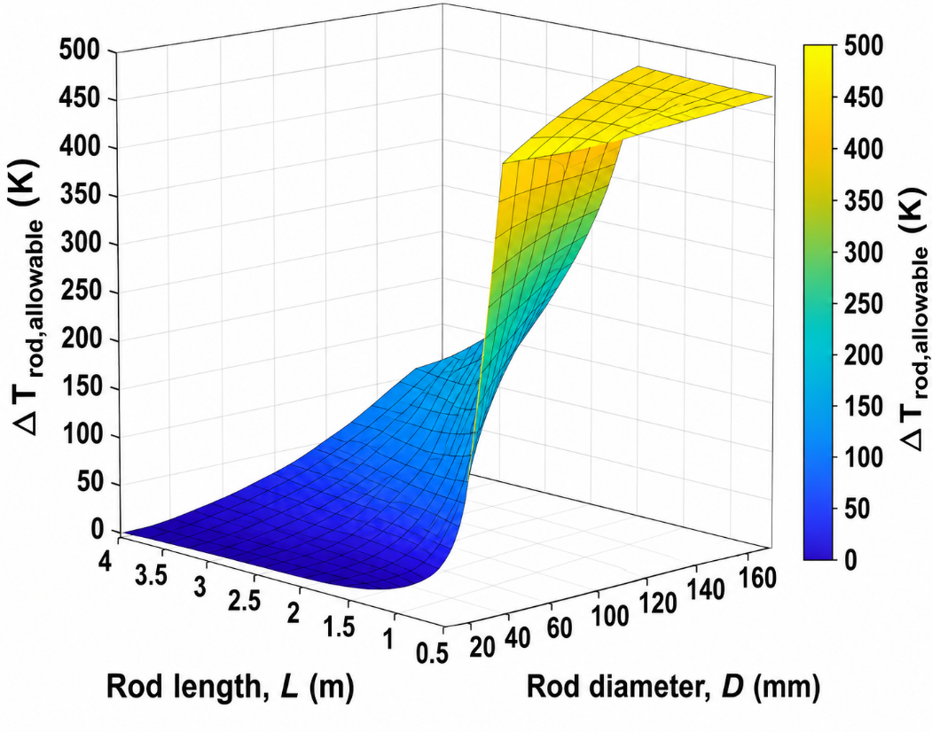
The feasible region in Figure 2 demonstrates that the admissible geometry contracts as the imposed temperature change increases. This behavior follows directly from the thermal-force relation in Eq. (4): for fixed geometry and load-transfer conditions, F_th increases linearly with ΔT_rod. Consequently, larger temperature excursions require either a larger diameter, a shorter rod, or a combination of both to maintain structural stability.

Rod length has a particularly strong influence on the feasible domain because the Euler critical load varies as 1/L² [14, 15]. Long, slender rods therefore become unstable at substantially lower thermal loads than shorter rods of the same diameter. In contrast, increasing D improves buckling resistance rapidly because the second moment of area of a solid circular section scales as D⁴. The resulting geometry-temperature interaction produces a curved feasibility boundary rather than a simple independent limit on D, L, or ΔT_rod.

This observation is important for thermoelastic energy harvesting because increasing L would otherwise appear advantageous through the thermal elongation relation ΔL₀ = αLΔT_rod. The additional displacement obtained from a longer rod is therefore accompanied by a progressively stronger structural penalty. The usable design domain is consequently determined by the interaction between thermal expansion and structural stability rather than by thermal displacement alone.

3.2. Governing Failure Modes.

The governing structural failure modes over the investigated design space are summarized in Figure 3.

Figure 3

Governing structural failure modes in the thermoelastic rod design space. The map distinguishes safe designs from regions governed by Euler buckling, material yielding, or simultaneous violation of both constraints.

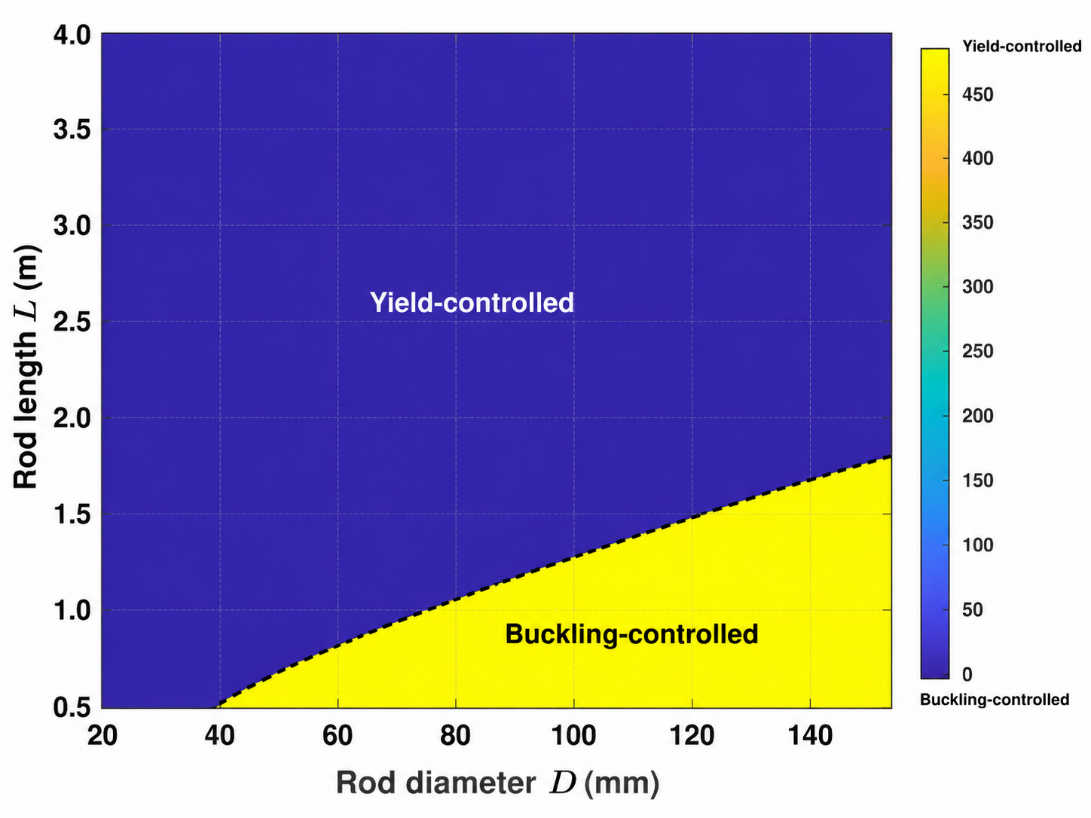
The failure map reveals two physically distinct structural limits. Buckling primarily controls the long and slender portion of the design domain, consistent with classical elastic-stability theory [14, 15]. Yielding, by contrast, is governed principally by the thermoelastic stress level. From Eq. (3), σ_th = λEαΔT_rod, showing that, within the present one-dimensional linear-elastic formulation, the nominal thermal stress is independent of rod diameter and length. The yield boundary is therefore driven predominantly by temperature change, material properties, load transfer, and the adopted safety factor rather than directly by rod geometry.

The difference between these two mechanisms explains the characteristic shape of the feasible region. Buckling introduces a strongly geometry-dependent boundary, whereas yielding imposes a predominantly temperature-dependent upper limit. Where both criteria are violated, increasing diameter alone may remove the buckling limitation but cannot eliminate a yield violation caused by excessive thermoelastic stress. This distinction is important when interpreting an optimization result: a geometry change can substantially improve stability against buckling, whereas a yield-controlled design requires modification of the thermal loading, restraint level, material strength, or safety criterion.

3.3. Effect of Temperature Change on Structural Feasibility

The evolution of the failure regions with temperature is examined more directly in Figure 4, which presents D - L failure maps at ΔT_rod = 50, 120, 300, and 500 K. These temperature levels were selected to illustrate the progressive transition from a predominantly buckling-limited domain toward increasingly severe material-strength restrictions.

Figure 4

Thermoelastic structural failure maps in the D - L design space at (a) ΔT_rod = 50 K, (b) ΔT_rod = 120 K, (c) ΔT_rod = 300 K, and (d) ΔT_rod = 500 K. Each map identifies safe, buckling-controlled, yield-controlled, and combined-failure regions under the same structural assumptions and safety factors.

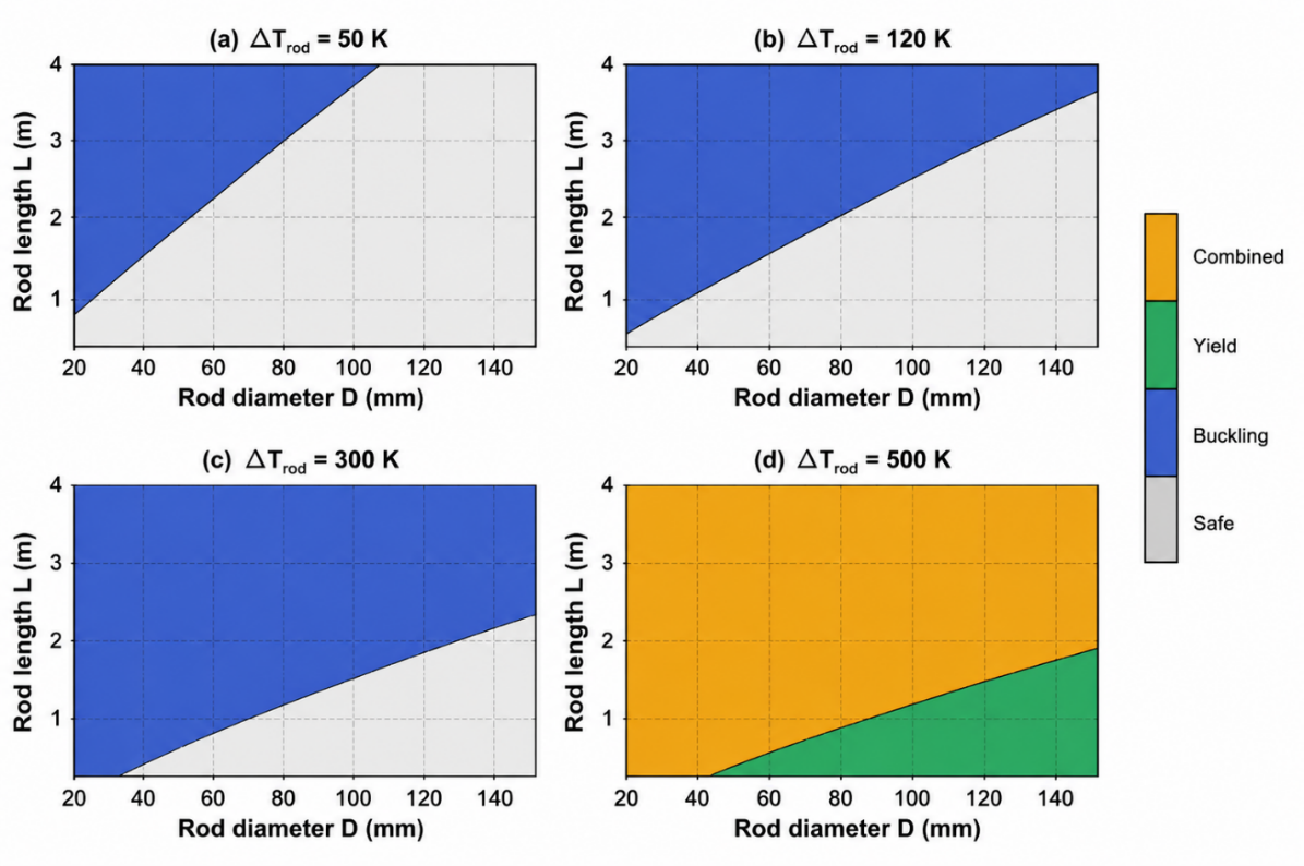
At ΔT_rod = 50 K, the thermal stress remains below the allowable yield limit for the investigated material and baseline restraint condition. The principal restriction is therefore Euler buckling, which eliminates sufficiently long and slender rods while leaving a comparatively broad safe region at larger diameters and shorter lengths.

At ΔT_rod = 120 K, the thermal force increases substantially and the buckling boundary moves toward larger diameters and shorter allowable lengths. Nevertheless, the design domain still contains a significant feasible region. This operating condition is therefore particularly useful for subsequent optimization because it provides a nontrivial trade-off between thermoelastic output and structural feasibility rather than an entirely unconstrained or entirely failure-dominated domain.

At ΔT_rod = 300 K, the structural margin becomes much smaller. Buckling continues to restrict slender geometries, while the thermoelastic stress approaches the allowable material-strength limit. The interaction between the two constraints therefore becomes increasingly important.

At ΔT_rod = 500 K, the yield criterion becomes dominant under the adopted linear-elastic material model and safety factor. Because the nominal thermoelastic stress in Eq. (3) does not decrease with increasing rod diameter, increasing D cannot by itself recover feasibility once the allowable stress has been exceeded. The high-temperature maps should therefore be interpreted primarily as a parametric demonstration of the transition between structural failure mechanisms rather than as a recommended operating range for AISI 4340 under the constant-property assumptions adopted here.

Taken together, Figures 2-4 show that the feasible design space is governed by a clear hierarchy of physical constraints. At relatively modest temperature changes, Euler buckling is the dominant limitation and strongly couples allowable rod length to diameter. As ΔT_rod increases, the admissible domain contracts until the material-strength criterion becomes increasingly important and ultimately dominant. These trends establish the structural basis for the mass-power optimization developed in Section 4: designs with high thermoelastic output cannot be selected independently of the stability boundary, and the resulting optimum is expected to lie close to an active structural constraint.

4.1. Mass–Power Trade-Off and Pareto Front

The feasible designs identified in Section 3 were evaluated in terms of structural mass and average mechanical power. The rod mass is calculated as:

where A is the cross-sectional area, and L is the rod length. The average mechanical power P_avg is obtained from Eq. (20).

These two performance measures are inherently conflicting. Increasing the rod dimensions can increase the mechanical work generated during a thermal cycle, but it also increases the material mass and thermal inertia. Consequently, maximizing P_avg alone favors substantially larger rods, whereas minimizing mass alone favors small geometries with limited power output. This constitutes a multi-objective optimization problem in which no single design simultaneously minimizes mass and maximizes power.

The feasible solutions were therefore screened using the Pareto-dominance principle [19, 20]. A design was classified as non-dominated when no other feasible design provided both lower mass and higher average power. The resulting mass-power Pareto front is shown in Figure 5.

Figure 5

Mass-power design space and Pareto front for the feasible thermoelastic rod configurations. Feasible solutions are shown together with the non-dominated Pareto designs, illustrating the trade-off between structural mass and average mechanical power.

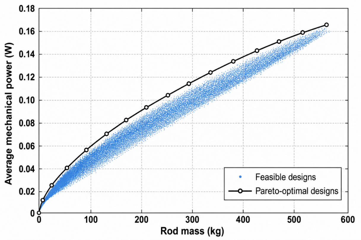
The Pareto front extends from a low-mass design of approximately 1.233 kg producing 0.002853 W to a maximum-power design of approximately 539.3 kg producing 0.16624 W under the baseline λ = 0.50 condition. Increasing mass therefore provides progressively greater average power, but the relationship is nonlinear and exhibits diminishing power gain per unit additional mass.

The numerical Pareto search produced 491 non-dominated designs for the 250 × 250 reference grid used in the detailed Pareto verification. An independent dominance check found no dominated points on the extracted front and no non-dominated feasible points outside it. The front can therefore be treated as the complete non-dominated set for the discretized design domain.

4.2. Buckling-Limited Energy–Power Scaling

The shape of the Pareto front can be interpreted analytically from the governing thermoelastic and structural relations. From Eq. (7), for fixed material properties, temperature change, and λ, the mechanical work scales as:

because A ∝ D² .

For the investigated convection-controlled thermal model, the characteristic thermal time increases approximately with the transverse dimension of the rod over the relevant geometry range. The average power therefore depends not only on the increase in mechanical work but also on the corresponding increase in cycle time. More importantly, the numerical Pareto solutions were found to lie predominantly close to the Euler-buckling boundary. Combining the thermal-force scaling:

with the Euler critical-load scaling [14, 15]

and imposing the active buckling condition F_th ∝ F_cr gives:

Thus, the buckling-limited Pareto designs maintain an approximately constant geometric slenderness. This behavior was confirmed numerically: the L/D ratio along the Pareto front remained approximately between 24.9 and 26.0, with a mean value of about 25.75, while most Pareto solutions were located close to the analytical buckling boundary. Because

and L ∝ D along the active buckling boundary,

or equivalently,

Along the buckling-limited family, for which L ∝ D, the lumped thermal time scale follows

whereas W ∝ D²L and L ∝ D give:

Therefore,

and substitution of D ∝ m^1/3 yields the principal scaling relation:

This result provides a physical interpretation of the Pareto front: under buckling-limited operation, average mechanical power increases sublinearly with structural mass. The analytical prediction was tested directly using the numerical Pareto solutions on logarithmic axes. The result is shown in Figure 6.

Figure 6

Log-log relationship between average mechanical power and rod mass along the Pareto front. The fitted power law closely follows the analytical scaling P_avg ∝ m^2/3 , confirming the buckling-controlled scaling behavior of the optimized thermoelastic rods.

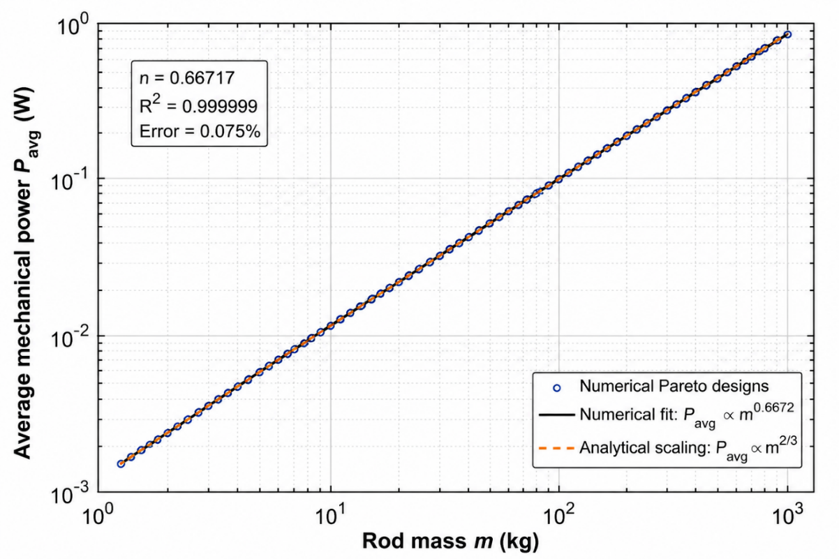
The numerical power-law fit can be expressed as:

with n = 0.66717 and C = 2.4967∙10^-3 W∙kg^-n for the units used in the present analysis. The fitted exponent differs from the theoretical value 2/3 by only approximately 0.075%, and the regression gives R² = 0.999999. The near-unity coefficient of determination indicates that the numerical Pareto front is extremely well represented by the predicted scaling law over the investigated domain.

This agreement is significant because Eq. (32) is not introduced as an empirical curve fit. It follows from the interaction between the thermoelastic work relation, convection-controlled thermal response, mass scaling, and the active Euler-buckling constraint. The numerical result therefore provides an independent verification of the analytical scaling argument.

4.3. Selection of a Compromise Design

Although every point on the Pareto front is non-dominated, engineering implementation generally requires selection of one representative design. A compromise solution was therefore identified using a normalized distance-to-ideal criterion, a commonly used approach in multi-objective decision making [19, 20, 21]. For each Pareto solution, mass and power were normalized over their respective Pareto ranges. Because mass is minimized whereas power is maximized, the normalized objectives were expressed as:

and

The Euclidean distance from the ideal point is then:

The compromise design is selected as the Pareto solution that minimizes the Euclidean distance d_ideal to the ideal point. The resulting selection is illustrated in Figure 7.

Figure 7

Selection of the compromise design from the mass-power Pareto front. (a) Location of the selected compromise design in the physical mass-power space. (b) Corresponding normalized Pareto representation and distance-to-ideal selection criterion.

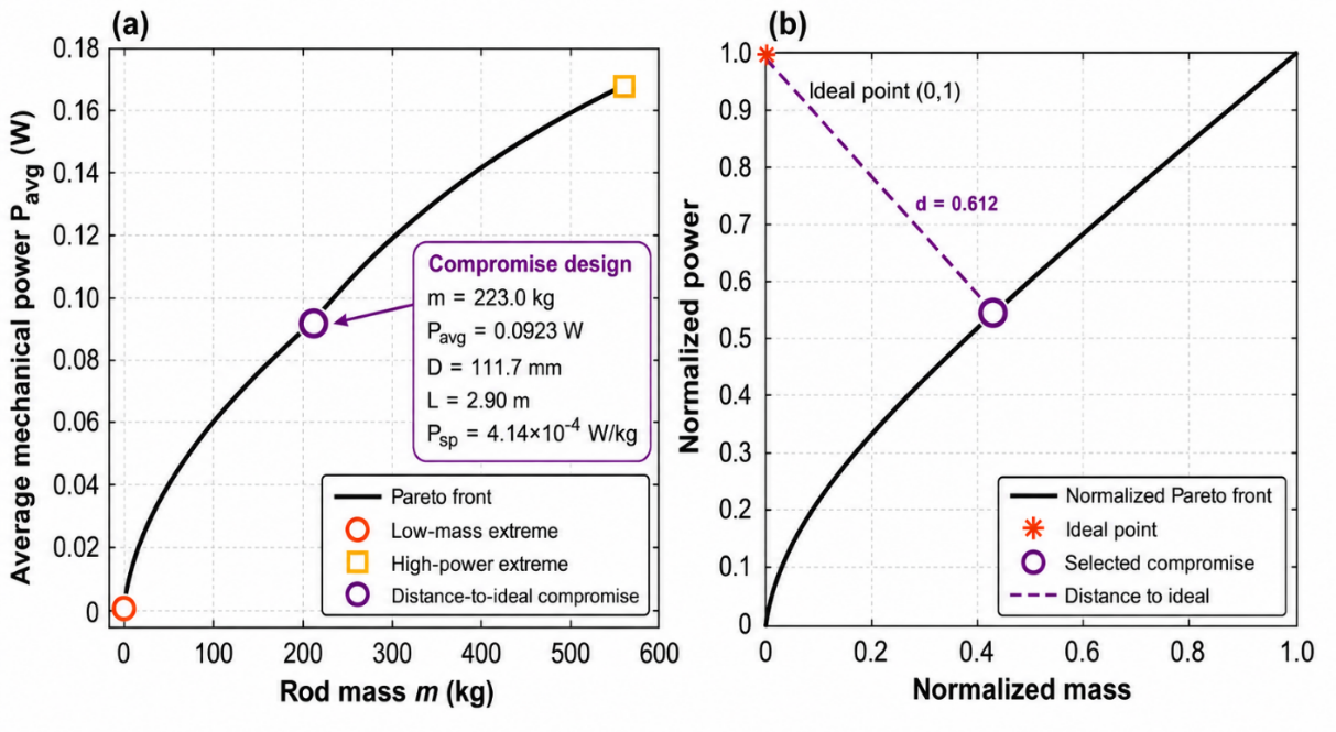
For the final 500 × 500 numerical grid, the distance-to-ideal method gives a compromise configuration with approximately: m = 223.0 kg; P_avg = 0.09231 W; D = 111.7 mm; L = 2.899 m. This design retains a substantial fraction of the maximum achievable power while avoiding the large mass associated with the extreme maximum-power configuration. By comparison, the baseline maximum-power design has D ≈ 150 mm, L ≈ 3.888 m, m ≈ 539.3 kg, and P_avg ≈ 0.16624 W. A second knee-point procedure based on the maximum perpendicular distance from the chord connecting the Pareto endpoints was also examined. However, numerical-resolution tests showed that this geometric knee location was substantially more sensitive to grid refinement than the distance-to-ideal solution. The distance-to-ideal method was therefore retained as the primary compromise-selection criterion, while the chord-distance method was used only as a robustness check. The principal optimization results are summarized in Table 3.

The results in Figures 5-7 demonstrate that the optimization is governed by a physically interpretable mass-power trade-off rather than by an isolated numerical maximum. The Pareto front is closely tied to the buckling boundary, its global trend follows the analytically predicted P_avg ∝ m^2/3 scaling law, and the distance-to-ideal criterion provides a reproducible intermediate design between the minimum-mass and maximum-power extremes. Sensitivity of these conclusions to heat transfer, λ, and numerical resolution is examined in Section 5.

5.1. Sensitivity to Convective Heat Transfer

The convective heat-transfer coefficient h directly controls the thermal response time of the rod and therefore has a strong influence on average mechanical power. Because h represents an external heat-transfer condition rather than a material property, its effect was evaluated over the range h = 10-100 W∙m^-2∙K^-1 while all other baseline parameters were held constant. From Eq. (16),

and because the temperature-response fraction ϕ is fixed, Eq. (19) gives:

For a fixed feasible geometry, the mechanical work W is independent of h in the present model. Therefore,

The numerical results confirm this expected linear dependence. The maximum average power increased from 0.033247 W at h = 10 W∙m^-2∙K^-1 to 0.166236 W at the baseline h = 50 W∙m^-2∙K^-1 and to 0.332471 W at h = 100 W∙m^-2∙K^-1. Over the same range, the cycle time of the maximum-power configuration decreased from approximately 80,785 s to 8,079 s.

Importantly, the maximum-power geometry remained essentially unchanged throughout this sensitivity range: D_opt = 150 mm; L_opt ≈ 3.888 m and the mechanical energy per cycle remained approximately 2686 J. Thus, within the present model, increasing h does not increase the mechanical energy obtained from an individual thermal cycle; instead, it allows essentially the same cycle to be completed more rapidly. This distinction explains the approximately proportional increase in average power.

The Biot number increases with h according to Eq. (12):

The maximum value in the investigated design domain increased from approximately 0.00827 at h = 10 W∙m^-2∙K^-1 to 0.08272 at h = 100 W∙m^-2∙K^-1. The latter value remains below the conventional Bi < 0.1 criterion for the lumped-capacitance approximation [16, 17]. Previous studies have also examined the validity and extension of lumped thermal models beyond this conventional range [18] and verified such formulations for different solid-fluid configurations [22]. Therefore, the lumped-capacitance approximation is considered appropriate for the parameter range investigated here. Conditions producing substantially larger h values would require renewed verification of the lumped-temperature assumption rather than simple extrapolation of Eq. (40).

5.2. Sensitivity to the Load-Transfer Parameter

The load-transfer parameter λ affects both useful displacement and compressive thermal force. For fixed geometry, Eq. (7) gives the mechanical-work dependence:

which has its unconstrained maximum at λ = 0.5. However, λ also enters the thermal force through Eq. (4). Increasing λ therefore raises the compressive force and reduces the maximum geometry that can satisfy the Euler-buckling constraint. Consequently, the system-level maximum-power value of λ need not coincide exactly with the fixed-geometry energy optimum. A refined sensitivity search was conducted over λ = 0.40-0.55 with Δλ = 0.001 using the final 500 × 500 geometry grid. The resulting power and geometry variations are shown in Figure 8.

Figure 8

Effect of the load-transfer parameter λ on the maximum achievable average mechanical power and the corresponding optimal rod geometry. (a) Maximum average power as a function of λ, showing the numerical optimum at λ_opt = 0.473 with P_max = 0.170454 W and the reference case λ = 0.500, for which P_max = 0.166245 W. (b) Corresponding optimal rod diameter D_opt and length L_opt over the investigated λ range. The optimal diameter remains at the upper design bound of 150 mm, whereas the optimal length decreases as the buckling constraint becomes increasingly restrictive.

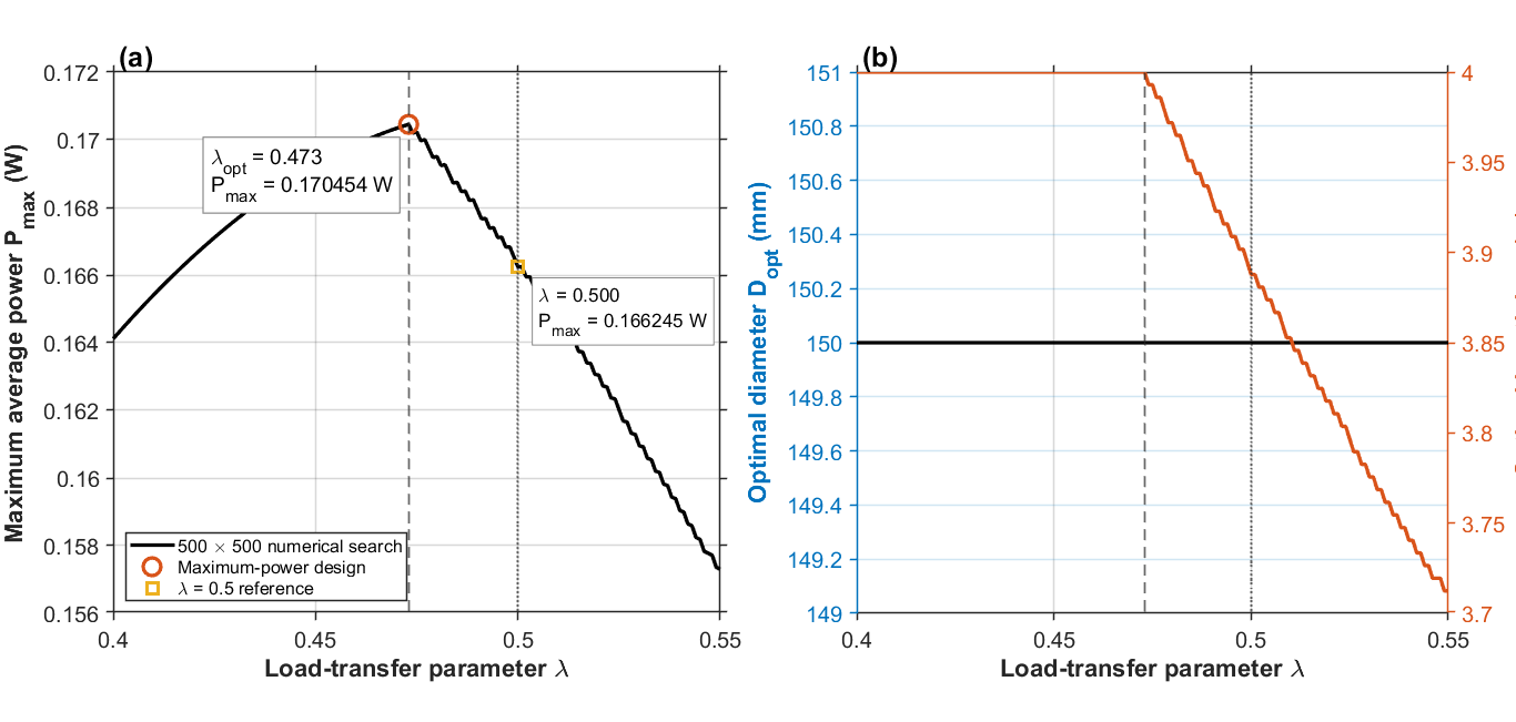
The refined numerical search gives λ_opt = 0.473 with P_max = 0.170454 W, D_opt = 150 mm, L_opt = 4.000 m and a corresponding rod mass of approximately 554.9 kg. At the baseline value λ = 0.500, the maximum average power is 0.166245 W. The relative power penalty associated with retaining the simple λ = 0.5 load-transfer condition is therefore only Power penalty = 2.47%.

The shift of the system optimum from 0.500 to approximately 0.473 has a clear structural origin. Up to the vicinity of the optimum, the maximum-power configuration remains at the imposed upper geometric limits D = 150 mm and L = 4.0 m. As λ increases further, the compressive thermal force becomes sufficiently large for Euler buckling to become active, forcing the optimal length below 4.0 m. The system optimum consequently occurs close to the transition between the geometry-bounded and buckling-bounded regimes. This result also clarifies the distinction between two different optimum definitions. The value λ = 0.5 remains the exact optimum of the fixed-geometry factor λ(1 − λ), whereas λ_opt ≈ 0.473 is the maximum-power solution of the bounded and structurally constrained system. The relatively small 2.47% difference in power indicates that λ = 0.5 remains a useful and robust baseline condition even though it is not the precise system-level optimum.

5.3. Grid-Convergence Verification

Because the Pareto front is obtained by discretizing the continuous D - L design domain, the influence of numerical resolution was evaluated using three successively refined grids: 125 × 125, 250 × 250 and 500 × 500. Grid convergence was assessed for both the maximum-power solution and the distance-to-ideal Pareto compromise. Numerical robustness is particularly important in multi-objective analysis because the extracted Pareto set and subsequent decision criterion should not depend strongly on arbitrary discretization choices [19, 20, 21, 22, 23].

The maximum-power result showed very rapid convergence. Between the 250 × 250 and 500 × 500 grids, the relative change in maximum power was only ΔP_max = 0.0057% while the change in the corresponding rod mass was Δm = 0.0058%. The distance-to-ideal compromise was also stable. Between the same two grids, the compromise mass changed by Δm_comp = 0.494% and the compromise power changed by ΔP_comp = 0.330%. The corresponding final 500 × 500 compromise configuration was approximately: m = 223.0 kg, P_avg = 0.09231 W, D = 111.7 mm and L = 2.899 m. These changes are sufficiently small to indicate that the principal maximum-power and compromise-design conclusions are insensitive to further refinement of the investigated discretization.

5.4. Pareto-Front and Compromise-Selection Robustness

The Pareto extraction procedure was independently checked for both internal non-dominance and completeness. For the 250 × 250 reference calculation, 30,480 feasible designs produced 491 Pareto-optimal points. A direct pairwise verification gave: Dominated points on Pareto front = 0 and: Non-dominated feasible points outside Pareto front = 0. Thus, within the discretized domain, the extraction algorithm neither retained dominated designs nor omitted non-dominated solutions.

The robustness of the compromise-design criterion was also examined using two independent approaches. The primary approach was the normalized distance-to-ideal method used in Section 4. A second geometric method identified the Pareto point with the maximum perpendicular distance from the chord connecting the two extreme solutions.

The two methods did not exhibit the same numerical stability. For the distance-to-ideal criterion, refinement from 250 × 250 to 500 × 500 changed the selected mass and power by only 0.494% and 0.330%, respectively. In contrast, the chord-distance method changed the selected mass by approximately 11.75% and the power by approximately 7.64%.

To determine whether this sensitivity was caused merely by nonuniform spacing of the discrete Pareto points, the Pareto curve was reparameterized by arc length and resampled uniformly before the chord-distance criterion was reapplied. For the 250 × 250 grid, raw and resampled chord-distance results differed by only approximately 0.03% in mass and 0.02% in power, showing that nonuniform point spacing was not the primary cause of the instability.

Even after uniform arc-length resampling, refinement from 250 × 250 to 500 × 500 produced changes of approximately 10.91% in selected mass and 7.10% in power. The chord-distance method was therefore classified as grid-sensitive for the present Pareto geometry and was not used as the primary design-selection criterion. The normalized distance-to-ideal method was retained because it demonstrated substantially better convergence and provides an explicit compromise between the two normalized objectives [19, 20, 21].

5.5. Overall Robustness of the Optimization

The combined sensitivity and numerical tests establish four principal robustness characteristics of the model. First, average power responds predictably to convective heat transfer, with Pmax varying approximately linearly with h while the maximum-power geometry remains nearly unchanged over the investigated range. Second, the lumped-capacitance approximation remains consistent with Bi < 0.1 throughout the tested convection domain. Third, refinement of λ confirms a reproducible system-level optimum near λ = 0.473, while the simpler λ = 0.5 condition incurs only a small power penalty. Fourth, both the maximum-power solution and the distance-to-ideal Pareto compromise are effectively grid-converged at the adopted numerical resolution.

The principal optimization and sensitivity values are summarized in Table 3. Collectively, these tests indicate that the central trends reported in Sections 3 and 4 are not artifacts of a single convection coefficient, a coarse geometry grid, or an arbitrary Pareto-selection procedure. The physical interpretation and limitations of these results are discussed in Section 6.

The results show that thermoelastic rod optimization is governed by a coupled structural-thermal trade-off rather than by thermal expansion alone. In the practically relevant part of the investigated domain, Euler buckling is the principal geometric constraint, forcing the high-performance Pareto solutions toward an approximately constant L/D ratio. This behavior explains the observed scaling P_avg ∝ m^2/3 and provides a physically interpretable design rule rather than a purely empirical numerical correlation. At larger temperature changes, yielding progressively replaces buckling as the governing constraint, consistent with classical thermoelastic and stability theory [6, 14, 15].

The optimization also demonstrates that maximum power should not be interpreted as the only useful design objective. The maximum-power configuration requires a comparatively large rod mass, whereas the distance-to-ideal solution provides a substantially lighter compromise with lower but still meaningful power output. The stability of this compromise under grid refinement strengthens its usefulness as an engineering design point. Likewise, the refined optimum λ = 0.473 differs only moderately from the analytically convenient λ = 0.5, for which the maximum-power penalty is approximately 2.47%.

Heat transfer remains a major practical limitation. Within the lumped model, P_avg ∝ h, because increasing h shortens the thermal cycle without changing the mechanical work per cycle. This prediction is valid only while the lumped-capacitance assumption remains applicable. The present calculations satisfy the conventional Bi < 0.1 criterion throughout the investigated range [16]. Nevertheless, the accuracy of lumped thermal models depends on the underlying heat-transfer conditions, and their applicability should be reassessed when these conditions change substantially [24]. Actual devices may exhibit nonuniform temperature fields, contact thermal resistance, variable convection, and temperature-dependent material properties, which are not represented by the present first-order thermal model.

Several additional limitations should therefore be recognized. The rod is treated as homogeneous, linearly elastic, and perfectly aligned, while Euler buckling is represented using ideal pinned-pinned boundary conditions. Joint compliance, friction, mechanical transmission losses, local stress concentrations, cyclic fatigue, imperfections, and heat losses to supporting structures are excluded. Consequently, the predicted mechanical power represents an idealized rod-level value rather than the net electrical output of a complete energy-harvesting device.

Despite these limitations, the model provides a useful first-stage design framework for identifying feasible geometries, governing failure modes, mass-power scaling, and robust compromise solutions before higher-fidelity simulation or experimental prototyping. Future validation should therefore focus on coupled transient thermo-mechanical analysis and experiments incorporating realistic supports, thermal contacts, mechanical transmission efficiency, and cyclic loading.

This study developed a coupled thermoelastic-structural-thermal framework for the constrained optimization of cylindrical thermoelastic energy-harvesting rods. The main conclusions are as follows:

Structural feasibility is governed primarily by Euler buckling at moderate temperature changes. Increasing the temperature excursion progressively contracts the feasible D-L domain, while yielding becomes increasingly important at higher thermal loads. The Pareto-optimal designs are concentrated close to the buckling boundary.

A clear mass-power scaling law emerges from the constrained design space. Analytical scaling predicts P_avg ∝ m^2/3 , while the numerical Pareto fit gives an exponent of 0.66717 with R² = 0.999999. The approximately 0.075% deviation from the theoretical exponent confirms that the observed scaling is a consequence of the governing thermoelastic, thermal, and buckling relations rather than a numerical artifact.

The mass-power Pareto front provides a practical alternative to single-objective maximum-power design. The distance-to-ideal criterion identifies a compromise configuration of approximately D = 111.7 mm and L = 2.899 m, with a mass of 223.0 kg and average mechanical power of 0.09231 W. This avoids the substantially larger mass associated with the baseline maximum-power configuration.

The load-transfer optimum is close to, but not exactly, λ = 0.5. Refined optimization gives λ_opt = 0.473, with P_max = 0.170454 W at D = 150 mm and L = 4.000 m. Using the analytically convenient baseline λ = 0.5 reduces the maximum power by only approximately 2.47%, indicating that λ = 0.5 remains a robust practical approximation.

The principal optimization results are numerically robust. Between the 250 × 250 and 500 × 500 grids, the maximum-power result changes by only approximately 0.006%, while the distance-to-ideal compromise changes by less than 0.5% in mass and 0.4% in power. Average power also exhibits the expected approximately linear dependence on the convective heat-transfer coefficient while the Biot number remains below 0.1 throughout the investigated range.

Overall, the results establish quantitative relationships among rod geometry, structural stability, thermal response, mass, and average mechanical power. The derived scaling law and Pareto framework provide compact design rules for preliminary thermoelastic energy-harvester optimization. Experimental validation and higher-fidelity transient thermo-mechanical modeling are required before the predicted rod-level performance can be translated into practical device-level electrical output.

References

- Kishore, R.A.; Priya, S. A Review on Low-Grade Thermal Energy Harvesting: Materials, Methods and Devices. Materials 2018, 11, 1433. https://doi.org/10.3390/ma11081433[CrossRef] [PubMed]
- Chen, H.; Goswami, D.Y.; Stefanakos, E.K. A Review of Thermodynamic Cycles and Working Fluids for the Conversion of Low-Grade Heat. Renewable and Sustainable Energy Reviews 2010, 14, 3059-3067. https://doi.org/10.1016/j.rser.2010.07.006[CrossRef]
- Tchanche, B.F.; Lambrinos, G.; Frangoudakis, A.; Papadakis, G. Low-Grade Heat Conversion into Power Using Organic Rankine Cycles—A Review of Various Applications. Renewable and Sustainable Energy Reviews 2011, 15, 3963-3979. https://doi.org/10.1016/j.rser.2011.07.024[CrossRef]
- Vélez, F.; Segovia, J.J.; Martín, M.C.; Antolín, G.; Chejne, F.; Quijano, A. A Technical, Economical and Market Review of Organic Rankine Cycles for the Conversion of Low-Grade Heat for Power Generation. Renewable and Sustainable Energy Reviews 2012, 16, 4175-4189. https://doi.org/10.1016/j.rser.2012.03.022[CrossRef]
- Kishore, R.A.; Davis, B.; Greathouse, J.; Hannon, A.; Kennedy, D.E.; Millar, A.; Mittel, D.; Nozariasbmarz, A.; Kang, M.G.; Kang, H.B.; Sanghadasa, M.; Priya, S. Energy Scavenging from Ultra-Low Temperature Gradients. Energy & Environmental Science 2019, 12, 1008-1018. https://doi.org/10.1039/C8EE03084G[CrossRef]
- Boley, B.A.; Weiner, J.H. Theory of Thermal Stresses; Dover Publications: Mineola, NY, USA, 1997.
- Dimitriev, O.P. Thermomechanical Energy Converters for Harvesting Thermal Energy: A Review. Journal of Renewable Materials 2023, 11(4), 1555-1600. DOI: 10.32604/jrm.2023.024772.[CrossRef]
- Kim, S.H.; Sim, H.J.; Hyeon, J.S.; Suh, D.; Spinks, G.M.; Baughman, R.H.; Kim, S.J. Harvesting Electrical Energy from Torsional Thermal Actuation Driven by Natural Convection. Scientific Reports 2018, 8, 8712. DOI: 10.1038/s41598-018-26983-4.[CrossRef] [PubMed]
- Oudich, A.; Thiebaud, F. A Two-Way Shape Memory Alloy-Piezoelectric Bimorph for Thermal Energy Harvesting. Mechanics of Materials 2016, 102, 1-6. DOI: 10.1016/j.mechmat.2016.08.006.[CrossRef]
- McKinley, I.M.; Lee, F.Y.; Pilon, L. A Novel Thermomechanical Energy Conversion Cycle. Applied Energy 2014, 126, 78-89. DOI: 10.1016/j.apenergy.2014.03.069.[CrossRef]
- Parsokhonov, A.; Nurullayev, O.; Akhmedov, A. An Alternative Renewable Energy Source: Thermal Expansion and Contraction of Materials. Online Journal of Engineering Sciences 2025, 4(1), 1-12. DOI: 10.31586/ojes.2025.6087.[CrossRef]
- Parsokhonov, A.G.; Nurullayev, O.U.; Akhmedov, A.A.; Olimov, O.O.; Kushakov, G.A. Scaling Laws and Thermodynamic Limits of Modular Thermoelastic Energy Harvesting from Low-Grade Heat. Energies 2026, 19, 3657. https://doi.org/10.3390/en19153657[CrossRef]
- Goh, W.L.; Zheng, Y.; Yuan, J.; Ng, K.W. Effects of Hardness of Steel on Ceramic Armour Module against Long Rod Impact. International Journal of Impact Engineering 2017, 109, 419-426. DOI: 10.1016/j.ijimpeng.2017.08.004.[CrossRef]
- Brush, D.O.; Almroth, B.O. Buckling of Bars, Plates, and Shells; McGraw-Hill: New York, NY, USA, 1975.[CrossRef]
- Timoshenko, S.P.; Gere, J.M. Theory of Elastic Stability, 2nd ed.; McGraw-Hill: New York, NY, USA, 1961.
- Incropera, F.P.; DeWitt, D.P.; Bergman, T.L.; Lavine, A.S. Fundamentals of Heat and Mass Transfer, 6th ed.; John Wiley & Sons: Hoboken, NJ, USA, 2007.
- Çengel, Y.A.; Ghajar, A.J. Heat and Mass Transfer: Fundamentals & Applications, 5th ed.; McGraw-Hill Education: New York, NY, USA, 2015.
- Xu, B.; Li, P.-W.; Chan, C.L. Extending the Validity of Lumped Capacitance Method for Large Biot Number in Thermal Storage Application. Solar Energy 2012, 86, 1709-1724. DOI: 10.1016/j.solener.2012.03.016.[CrossRef]
- Deb, K. Multi-Objective Optimization Using Evolutionary Algorithms; John Wiley & Sons: Chichester, UK, 2001.
- Miettinen, K. Nonlinear Multiobjective Optimization; Kluwer Academic Publishers: Boston, MA, USA, 1999.
- Marler, R.T.; Arora, J.S. Survey of Multi-Objective Optimization Methods for Engineering. Structural and Multidisciplinary Optimization 2004, 26, 369-395. DOI: 10.1007/s00158-003-0368-6.[CrossRef]
- Li, P.; Xu, B.; Han, J.; Yang, Y. Verification of a Model of Thermal Storage Incorporated with an Extended Lumped Capacitance Method for Various Solid-Fluid Structural Combinations. Solar Energy 2014, 105, 71-81. DOI: 10.1016/j.solener.2014.03.038.[CrossRef]
- Giannelos, S.; Zhang, X.; Zhang, T.; Strbac, G. Multi-Objective Optimization for Pareto Frontier Sensitivity Analysis in Power Systems. Sustainability 2024, 16, 5854. DOI: 10.3390/su16145854.[CrossRef]
- Campo, A. The Lumped Capacitance Model for Unsteady Heat Conduction in Regular Solid Bodies With Natural Convection to Nearby Fluids Engages the Nonlinear Bernoulli Equation. Journal of Thermal Science and Engineering Applications 2018, 10(3). DOI: 10.1115/1.4038539.[CrossRef]